Welcome to SKLearn 101! In this post, we will introduce scikit-learn, an open-source machine learning toolkit that is essential for any data scientist or machine learning practitioner.
We will use the World Happiness Report dataset to explore one of the most common applications of statistical modeling: Linear Regression. Linear regression helps estimate the relationship between an independent variable (explanatory variable) and a dependent variable (response).
1. Import the Libraries
As usual, we first import the necessary libraries. We’ll use pandas for data manipulation, matplotlib and seaborn for visualization, and sklearn for our machine learning models.
import pandas as pd
import numpy as np
import matplotlib.pyplot as plt
import seaborn as sns

# Import various functions from scikit-learn to help with the model
from sklearn.linear_model import LinearRegression
from sklearn.model_selection import train_test_split
from sklearn import metrics
2. Import and Process the Data
The World Happiness dataset contains various metrics for different countries over several years. We’ll start by loading the data, cleaning column names, and dropping missing values.
# Open the dataset
df = pd.read_csv('world_happiness.csv')

# Rename the column names so they don't contain spaces
df = df.rename(columns={i: "_".join(i.split(" ")).lower() for i in df.columns})

# Drop all of the rows which contain empty values
df = df.dropna()

# Show the first few rows
df.head()
The dataset includes columns like life_ladder (subjective life quality), log_gdp_per_capita, social_support, healthy_life_expectancy_at_birth, and more.
3. Inspect the Data
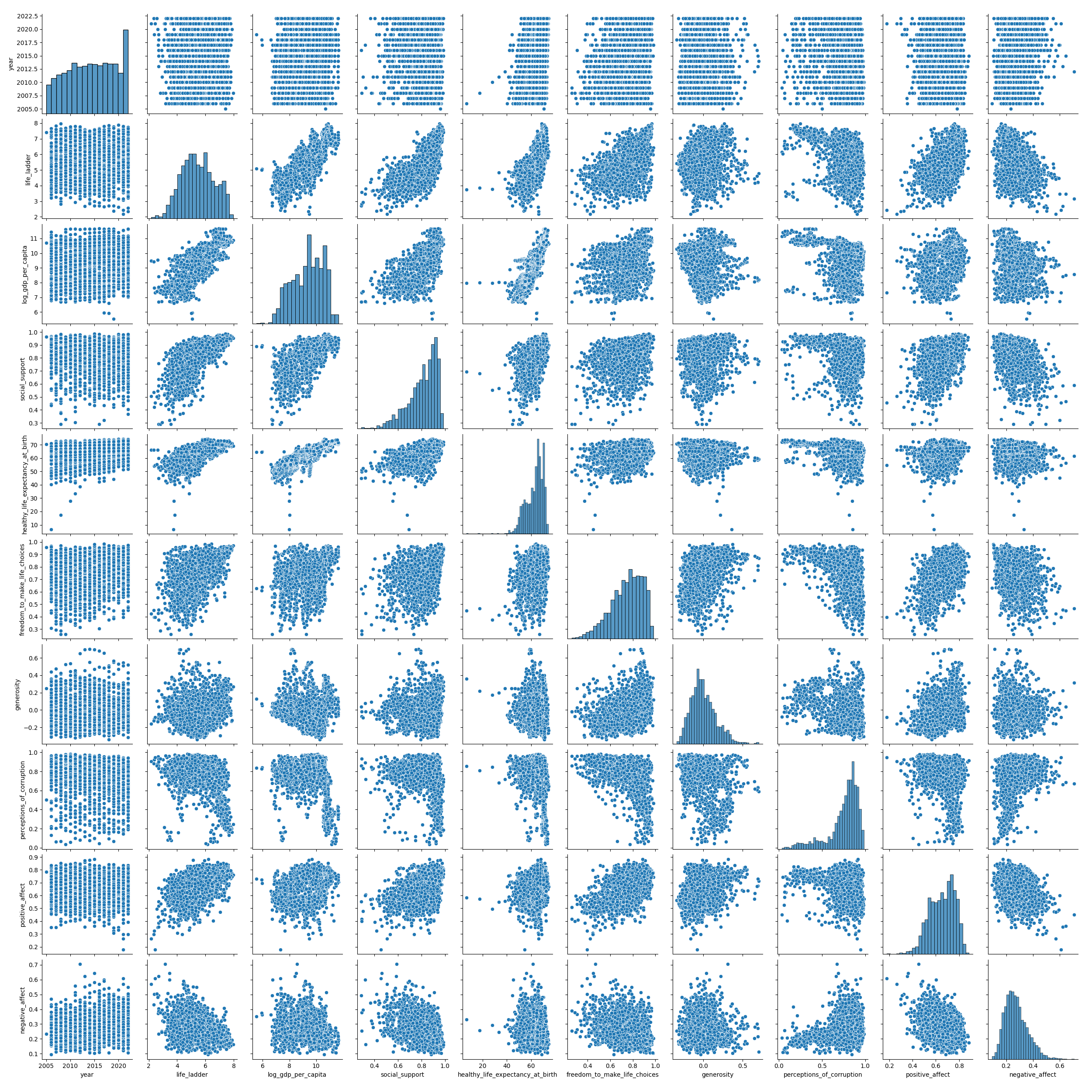
Before fitting a model, it’s important to visualize the data. A pairplot is a great way to see scatter plots between each pair of columns and histograms for each individual column.
# Visualize the data using seaborn
sns.pairplot(df)
4. Simple Linear Regression
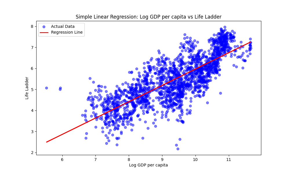
In simple linear regression, we use one independent variable to predict a response. Let’s start by trying to predict the life_ladder score using only log_gdp_per_capita.
# Define the explanatory (X) and response (y) variables
X = df[['log_gdp_per_capita']]
y = df['life_ladder']

# Initialize and fit the model
model = LinearRegression()
model.fit(X, y)

# Make predictions
y_pred = model.predict(X)
We can visualize the fit by plotting the regression line over the original data.
5. Multiple Linear Regression
What if we want to use more than one variable to predict happiness? In multiple linear regression, we incorporate multiple explanatory variables.
# Define multiple explanatory variables
X = df[['log_gdp_per_capita', 'social_support', 'healthy_life_expectancy_at_birth',
        'freedom_to_make_life_choices', 'generosity', 'perceptions_of_corruption']]
y = df['life_ladder']

# Fit the multiple linear regression model
model_multi = LinearRegression()
model_multi.fit(X, y)

# Get the coefficients (weights) for each variable
pd.DataFrame(model_multi.coef_, X.columns, columns=['Coefficient'])
6. Model Evaluation
To understand how well our model is performing, we can look at metrics like the Mean Squared Error (MSE) and the Coefficient of Determination ($R^2$).
# Predict using the multiple regression model
y_pred_multi = model_multi.predict(X)

print('Mean Squared Error:', metrics.mean_squared_error(y, y_pred_multi))
print('R-squared:', metrics.r2_score(y, y_pred_multi))
The $R^2$ score tells us the proportion of the variance in the dependent variable that is predictable from the independent variables. A higher $R^2$ generally indicates a better fit.
Summary
In this post, we’ve seen how to:
- Load and clean data using Pandas.
- Visualize relationships using Seaborn.
- Fit simple and multiple linear regression models using Scikit-Learn.
- Evaluate model performance using standard metrics.
Stay tuned for the next post in the SKLearn 101 series!