Probability 104: Central Limit Theorem

Welcome back! In our previous post, we explored dice simulations and saw a hint of a powerful statistical concept. Today, we’re diving deep into the Central Limit Theorem (CLT)—one of the most important theorems in statistics.

The CLT states that the sum or average of a large number of independent and identically distributed (i.i.d.) random variables tends to follow a normal distribution, regardless of the original distribution of the variables themselves.

Let’s see the theorem in action! 📊✨

Setting Up

We’ll use numpy for simulations and seaborn/matplotlib for visualization.

import numpy as np
import pandas as pd
import seaborn as sns
import matplotlib.pyplot as plt
from scipy import stats
from scipy.stats import norm

1. Gaussian Population

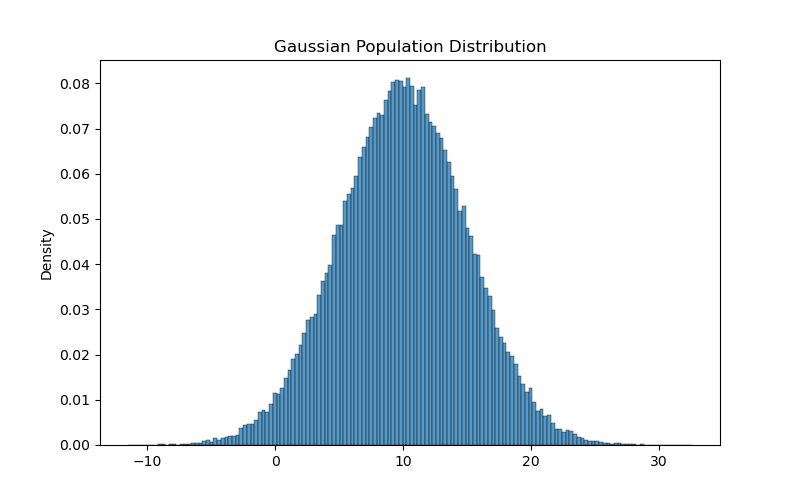
We’ll begin with the most straightforward scenario: when your population follows a Gaussian distribution.

mu = 10
sigma = 5

gaussian_population = np.random.normal(mu, sigma, 100_000)

The population has a mean of 10 and a standard deviation of 5. You can visualize its histogram below:

Estimating Population Parameters

If you didn’t know the values of $\mu$ and $\sigma$, you could estimate them by computing the mean and standard deviation of the whole population:

gaussian_pop_mean = np.mean(gaussian_population)
gaussian_pop_std = np.std(gaussian_population)

print(f"Gaussian population has mean: {gaussian_pop_mean:.1f} and std: {gaussian_pop_std:.1f}")

Output:

Gaussian population has mean: 10.0 and std: 5.0

Sampling from the Population

In real life, you won’t have access to the whole population. This is where sampling comes in. We’ll define a function to take random samples (with replacement) and compute their means.

def sample_means(data, sample_size):
    # Save all the means in a list
    means = []

    # Take 10,000 samples
    for _ in range(10_000):
        # Get a sample of the data WITH replacement
        sample = np.random.choice(data, size=sample_size)
        # Save the mean of the sample
        means.append(np.mean(sample))

    return np.array(means)

CLT in Action (Gaussian)

The theorem states that if a large enough sample_size is used, the distribution of the sample means should be Gaussian. Even with a small size ($n=5$), the distribution looks pretty Gaussian:

# Compute the sample means
gaussian_sample_means = sample_means(gaussian_population, sample_size=5)

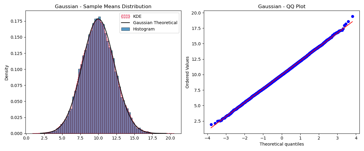
The QQ Plot (right) yields an almost perfect straight line, confirming the sample means follow a Gaussian distribution.

2. Binomial Population

Now let’s try with a distribution that is not Gaussian: the Binomial distribution.

n = 5
p = 0.8

binomial_population = np.random.binomial(n, p, 100_000)

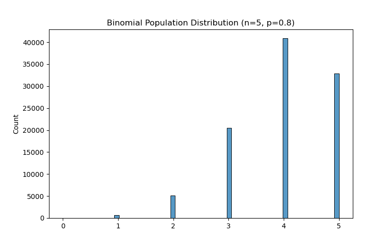
We can compute the population parameters directly or use formulas ($\mu = np$, $\sigma = \sqrt{np(1-p)}$):

binomial_pop_mean = n * p
binomial_pop_std = np.sqrt(n * p * (1 - p))

print(f"Binomial population has mean: {binomial_pop_mean:.1f} and std: {binomial_pop_std:.1f}")

Output:

Binomial population has mean: 4.0 and std: 0.9

The Rule of Thumb

For the Binomial distribution, a rule of thumb to know if the CLT will hold is: $if \ \min(Np, N(1-p)) \ge 5 \ \text{then CLT holds}$ (where $N = n \cdot \text{sample\_size}$)

Small Sample Size ($n=3$)

sample_size = 3
N = n * sample_size

condition_value = np.min([N * p, N * (1 - p)])
print(f"The condition value is: {int(condition_value*10)/10:.1f}. CLT should hold?: {condition_value >= 5}")

Output:

The condition value is: 3.0. CLT should hold?: False

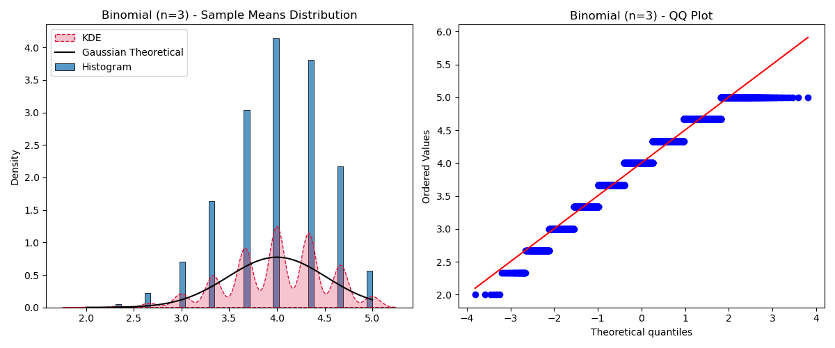
With $n=3$, the distribution is discrete and skewed. The KDE doesn’t match the Gaussian well.

Large Sample Size ($n=30$)

sample_size = 30
# ... compute means ...

Output:

The condition value is: 30.0. CLT should hold?: True

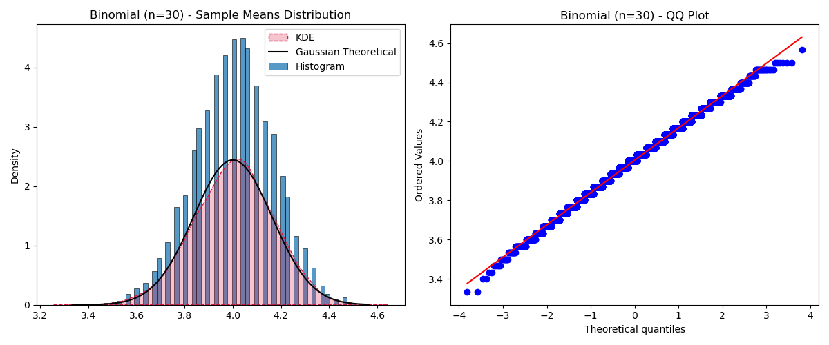
Now the theorem holds beautifully!

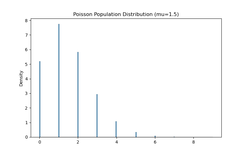
3. Poisson Population

The Poisson distribution models the number of events in a fixed interval. It has a mean and variance both equal to $\mu$.

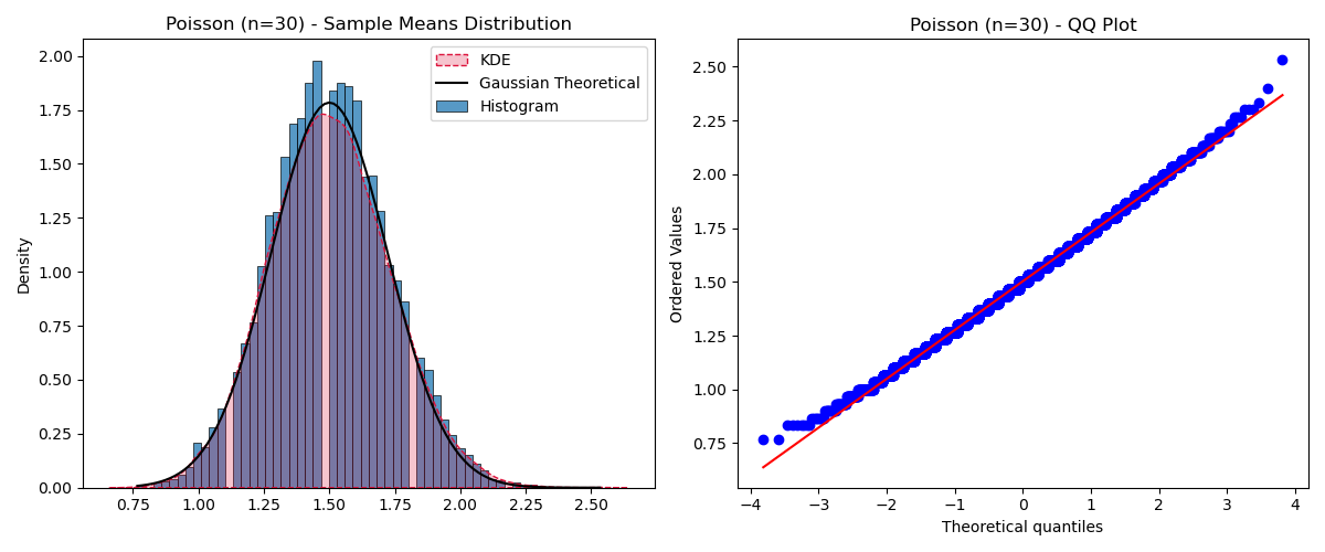
With a sample size of $n=30$, the sample means clearly converge to a Gaussian distribution.

4. When CLT Fails: Cauchy Distribution

The CLT requires the distribution to have a finite mean and variance. The Cauchy Distribution has “heavy tails” and neither a well-defined mean nor variance.

cauchy_population = np.random.standard_cauchy(1000)

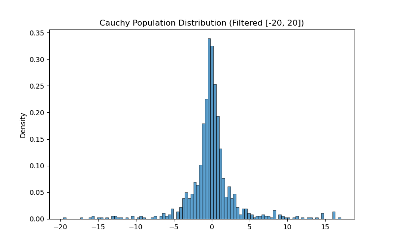
Let’s look at the QQ plot for sample means even with large $n$:

$n=30$	$n=100$

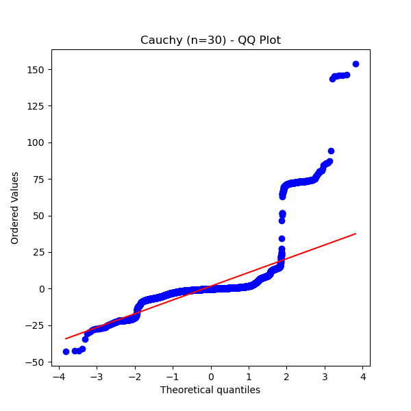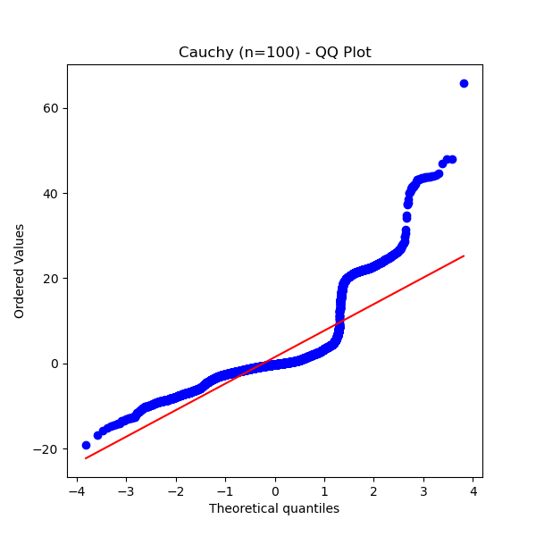Even with $n=100$, the QQ plot is nowhere near a straight line. The extreme values continue to pull the mean away from normality.

Summary

The Central Limit Theorem is the reason why we see the “Bell Curve” everywhere.

• CLT Holds: When variables are independent and have finite mean and variance. Rule of thumb: $n \ge 30$.
• CLT Fails: For distributions with infinite/undefined variance (like Cauchy).

Understanding these boundaries is key to applying statistical inference correctly!

Happy sampling! 📈🎲