Welcome back! In our previous posts, we’ve explored the counter-intuitive world of probability through the Monty Hall Problem and Birthday Problems. Today, we’re taking a more hands-on approach by building dice simulations using Python and NumPy.
Simulations are incredibly powerful because they allow us to approximate theoretical results and visualize distributions without complex analytical derivations (though we’ll check those too!).
Let’s get started dice rolling! 🎲🤖
Setting Up or Simulation
We’ll use numpy for the core simulation logic, and seaborn alongside matplotlib to visualize our results.
import numpy as np
import seaborn as sns
import matplotlib.pyplot as plt

# Set seed for reproducibility
np.random.seed(42)
Representing a Die
The first step is to represent our die. For a standard 6-sided die, we can simply use a NumPy array containing the numbers 1 through 6.
# Define the desired number of sides
n_sides = 6

# Represent a die by using a numpy array
dice = np.array([i for i in range(1, n_sides+1)])

print(f"Our die: {dice}")
Rolling the Die
If we assume a fair die, the probability of landing on each side is the same ($1/6 \approx 0.167$), following a discrete uniform distribution. We can simulate a single roll using np.random.choice.
# Roll the die once
result = np.random.choice(dice)
print(f"Result of one roll: {result}")
To roll the die multiple times, we can specify a size or use a list comprehension. Let’s roll it 20 times and see what we get.
# Roll the die 20 times
n_rolls = 20
rolls = np.array([np.random.choice(dice) for _ in range(n_rolls)])

print(f"Results of 20 rolls: {rolls}")
print(f"Mean of rolls: {np.mean(rolls):.2f}")
print(f"Variance of rolls: {np.var(rolls):.2f}")
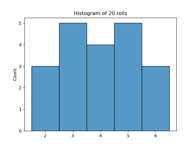
Visualizing 20 Rolls
Even with a fair die, a small number of trials (like 20) often won’t look perfectly uniform because of randomness.
The Law of Large Numbers
What happens if we roll the die 20,000 times? According to the Law of Large Numbers, as the number of trials increases, the experimental mean and distribution will converge to the theoretical values.
For a fair 6-sided die:
- Theoretical Mean: $(1+2+3+4+5+6)/6 = 3.5$
- Theoretical Variance: $\approx 2.917$
n_rolls = 20_000
rolls = np.array([np.random.choice(dice) for _ in range(n_rolls)])

print(f"Mean of 20k rolls: {np.mean(rolls):.2f}")
print(f"Variance of 20k rolls: {np.var(rolls):.2f}")
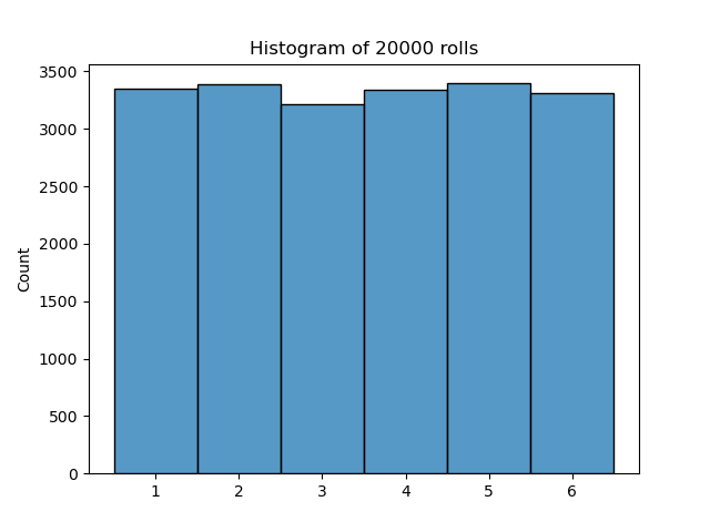
Now that looks much more like a uniform distribution!
Summing the Results of Rolling Twice
Suppose we roll two dice and record the sum. This is a classic probability problem (think Settlers of Catan!). Using NumPy’s vectorized operations, we can simulate this very efficiently.
n_rolls = 20_000

# Roll two sets of 20,000 trials
first_rolls = np.array([np.random.choice(dice) for _ in range(n_rolls)])
second_rolls = np.array([np.random.choice(dice) for _ in range(n_rolls)])

# Sum them element-wise
sum_of_rolls = first_rolls + second_rolls
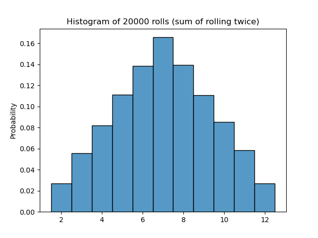
The resulting distribution looks “triangular” or approximately Gaussian (Bell Curve). This is a glimpse of the Central Limit Theorem in action: the sum of independent random variables tends toward a normal distribution.
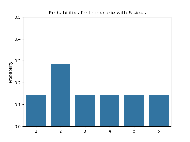
Simulating a Loaded Die
What if the die isn’t fair? Imagine a “loaded” die where one side is more likely to appear than others. np.random.choice allows us to pass a p parameter to define custom probabilities.
Suppose we want side 2 to be twice as likely as any other side.
Defining Probabilities
If we have $n$ sides and one side is twice as likely, we solve for $p$: $(n-1) \cdot p + 2p = 1 \implies (n+1)p = 1 \implies p = 1/(n+1)$.
For $n=6$, the standard sides get $1/7 \approx 0.143$, and the loaded side gets $2/7 \approx 0.286$.
def load_dice(n_sides, loaded_number):
    # All probabilities are initially 1/(n+1)
    probs = np.array([1/(n_sides+1) for _ in range(n_sides)])

    # The loaded side gets the remaining probability (which will be 2/(n+1))
    probs[loaded_number-1] = 1 - sum(probs[:-1])

    return probs

probs_loaded = load_dice(6, loaded_number=2)
print(f"Loaded probabilities: {probs_loaded}")
Rolling the Loaded Die
Now we simulate 20,000 rolls with these custom probabilities.
rolls_loaded = np.random.choice(dice, size=20_000, p=probs_loaded)
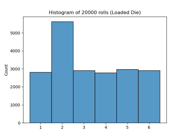
As expected, side 2 appears much more frequently than the others!
Conclusion
NumPy makes it incredibly easy to perform large-scale simulations. Whether you’re verifying the Law of Large Numbers or modeling complex “loaded” scenarios, rolling dice in code is a great way to build your intuition for probability.
Happy coding! 🎲