Welcome to Pandas 101! In this post, we will introduce the Pandas library, one of the most powerful tools for data analysis in Python. We will use the World Happiness Report dataset to demonstrate common operations like loading data, viewing data, selecting columns and rows, filtering, and basic plotting.
1. Importing the Libraries
The first step in any data analysis project is to import the necessary libraries. For this tutorial, we will need pandas for data manipulation and seaborn for additional visualization tools later on.
import pandas as pd
import seaborn as sns
2. Importing the Data
We will use a CSV file containing data from the World Happiness Report. We can load this into a Pandas DataFrame using the read_csv function.
# Import the data
df = pd.read_csv("world_happiness.csv")
3. Basic Operations With a Dataframe
3.1 View the Dataframe
Once the data is loaded, it’s a good idea to take a quick look at it. You can use the .head() and .tail() methods to see the first and last few rows of the DataFrame.
# Show the first 5 rows of the dataframe
df.head()
| Country name | year | Life Ladder | Log GDP per capita | Social support | Healthy life expectancy at birth | Freedom to make life choices | Generosity | Perceptions of corruption | Positive affect | Negative affect | |
|---|---|---|---|---|---|---|---|---|---|---|---|
| 0 | Afghanistan | 2008 | 3.724 | 7.350 | 0.451 | 50.5 | 0.718 | 0.168 | 0.882 | 0.414 | 0.258 |
| 1 | Afghanistan | 2009 | 4.401 | 7.508 | 0.552 | 50.8 | 0.679 | 0.191 | 0.850 | 0.481 | 0.237 |
| 2 | Afghanistan | 2010 | 4.758 | 7.613 | 0.539 | 51.1 | 0.600 | 0.123 | 0.707 | 0.517 | 0.275 |
| 3 | Afghanistan | 2011 | 3.832 | 7.581 | 0.521 | 51.4 | 0.496 | 0.166 | 0.731 | 0.430 | 0.267 |
| 4 | Afghanistan | 2012 | 3.783 | 7.661 | 0.521 | 51.7 | 0.531 | 0.238 | 0.776 | 0.614 | 0.268 |
Similarly, we can view the last 5 rows, or specify the number of rows we want to see.
# Show the last 2 rows of the dataframe
df.tail(2)
| Country name | year | Life Ladder | Log GDP per capita | Social support | Healthy life expectancy at birth | Freedom to make life choices | Generosity | Perceptions of corruption | Positive affect | Negative affect | |
|---|---|---|---|---|---|---|---|---|---|---|---|
| 2197 | Zimbabwe | 2021 | 3.155 | 7.657 | 0.685 | 54.050 | 0.668 | -0.076 | 0.757 | 0.610 | 0.242 |
| 2198 | Zimbabwe | 2022 | 3.296 | 7.670 | 0.666 | 54.525 | 0.652 | -0.070 | 0.753 | 0.641 | 0.191 |
3.2 Index and Column Names
In a DataFrame, data is stored in a two-dimensional grid. The rows are indexed and the columns are named. You can access these using df.index and df.columns.
df.index
RangeIndex(start=0, stop=2199, step=1)
df.columns
Index(['Country name', 'year', 'Life Ladder', 'Log GDP per capita', 'Social support', 'Healthy life expectancy at birth', 'Freedom to make life choices', 'Generosity', 'Perceptions of corruption', 'Positive affect', 'Negative affect'], dtype='object')
Renaming Columns
It is often useful to rename columns to remove spaces or make them more consistent. Here is a way to automatically replace spaces with underscores and convert names to lowercase:
# Create a dictionary mapping old column names to new column names
columns_to_rename = {i: "_".join(i.split(" ")).lower() for i in df.columns}

# Rename the columns
df = df.rename(columns=columns_to_rename)
df.head()
| country_name | year | life_ladder | log_gdp_per_capita | social_support | healthy_life_expectancy_at_birth | freedom_to_make_life_choices | generosity | perceptions_of_corruption | positive_affect | negative_affect | |
|---|---|---|---|---|---|---|---|---|---|---|---|
| 0 | Afghanistan | 2008 | 3.724 | 7.350 | 0.451 | 50.5 | 0.718 | 0.168 | 0.882 | 0.414 | 0.258 |
| 1 | Afghanistan | 2009 | 4.402 | 7.509 | 0.552 | 50.8 | 0.679 | 0.191 | 0.850 | 0.481 | 0.237 |
| 2 | Afghanistan | 2010 | 4.758 | 7.614 | 0.539 | 51.1 | 0.600 | 0.121 | 0.707 | 0.517 | 0.275 |
| 3 | Afghanistan | 2011 | 3.832 | 7.581 | 0.521 | 51.4 | 0.496 | 0.164 | 0.731 | 0.480 | 0.267 |
| 4 | Afghanistan | 2012 | 3.783 | 7.661 | 0.521 | 51.7 | 0.531 | 0.238 | 0.776 | 0.614 | 0.268 |
3.3 Data Types
Each column in a Pandas DataFrame has a specific data type (dtype). This allows different types of data to coexist in the same table.
df.dtypes
country_name                         object
year                                  int64
life_ladder                         float64
log_gdp_per_capita                  float64
social_support                      float64
healthy_life_expectancy_at_birth    float64
freedom_to_make_life_choices        float64
generosity                          float64
perceptions_of_corruption           float64
positive_affect                     float64
negative_affect                     float64
dtype: object
You can also change the data types if necessary using .astype():
# Change the type of all float columns to float
float_columns = [i for i in df.columns if i not in ["country_name", "year"]]
df = df.astype({i: float for i in float_columns})
Finally, df.info() gives a concise summary of the DataFrame, including the number of non-null values.
df.info()
<class 'pandas.core.frame.DataFrame'>
RangeIndex: 2199 entries, 0 to 2198
Data columns (total 11 columns):
 #   Column                            Non-Null Count  Dtype
---  ------                            --------------  -----
 0   country_name                      2199 non-null   object
 1   year                              2199 non-null   int64
 2   life_ladder                       2199 non-null   float64
 3   log_gdp_per_capita                2179 non-null   float64
 4   social_support                    2186 non-null   float64
 5   healthy_life_expectancy_at_birth  2145 non-null   float64
 6   freedom_to_make_life_choices      2166 non-null   float64
 7   generosity                        2126 non-null   float64
 8   perceptions_of_corruption         2083 non-null   float64
 9   positive_affect                   2175 non-null   float64
 10  negative_affect                   2183 non-null   float64
dtypes: float64(9), int64(1), object(1)
memory usage: 189.1+ KB
3.4 Selecting Columns
One way of selecting a single column is to use df.column_name. This returns a Pandas Series.
# Select the life_ladder column
x = df.life_ladder
print(f"type(x):\n {type(x)}\n")
type(x):
 <class 'pandas.core.series.Series'>
Another way is to use square brackets and the column name as a string:
x = df["life_ladder"]
Passing a list of labels rather than a single label selects multiple columns and returns a DataFrame:
# Selecting multiple columns
x = df[["life_ladder", "year"]]
3.5 Selecting Rows
You can use slicing to select a range of rows. This returns a DataFrame containing all columns for the specified rows.
# Select rows 2, 3, and 4
df[2:5]
| country_name | year | life_ladder | log_gdp_per_capita | social_support | healthy_life_expectancy_at_birth | freedom_to_make_life_choices | generosity | perceptions_of_corruption | positive_affect | negative_affect | |
|---|---|---|---|---|---|---|---|---|---|---|---|
| 2 | Afghanistan | 2010 | 4.758 | 7.614 | 0.539 | 51.1 | 0.600 | 0.121 | 0.707 | 0.517 | 0.275 |
| 3 | Afghanistan | 2011 | 3.832 | 7.581 | 0.521 | 51.4 | 0.496 | 0.164 | 0.731 | 0.480 | 0.267 |
| 4 | Afghanistan | 2012 | 3.783 | 7.661 | 0.521 | 51.7 | 0.531 | 0.238 | 0.776 | 0.614 | 0.268 |
3.6 Iterating Over Rows
If you need to iterate through the data row by row, you can use .iterrows(). It returns an index and a Series for each row.
index, row = next(df.iterrows())
print(row)
country_name                        Afghanistan
year                                       2008
life_ladder                               3.724
log_gdp_per_capita                         7.35
social_support                            0.451
healthy_life_expectancy_at_birth           50.5
freedom_to_make_life_choices              0.718
generosity                                0.168
perceptions_of_corruption                 0.882
positive_affect                           0.414
negative_affect                           0.258
Name: 0, dtype: object
3.7 Boolean Indexing
Boolean indexing allows you to filter the DataFrame based on conditions. For example, selecting data only for the year 2022:
# Select rows where the year is 2022
df_2022 = df[df["year"] == 2022]
After filtering, the index will still have its original values. You can reset the index using .reset_index(drop=True):
df_2022 = df_2022.reset_index(drop=True)
4. Summary Statistics
Pandas provides a quick way to calculate summary statistics for all numeric columns using .describe().
df.describe()
| year | life_ladder | log_gdp_per_capita | social_support | healthy_life_expectancy_at_birth | freedom_to_make_life_choices | generosity | perceptions_of_corruption | positive_affect | negative_affect | |
|---|---|---|---|---|---|---|---|---|---|---|
| count | 2199.000000 | 2199.000000 | 2179.000000 | 2186.000000 | 2145.000000 | 2166.000000 | 2126.000000 | 2083.000000 | 2175.000000 | 2183.000000 |
| mean | 2014.161437 | 5.479227 | 9.389760 | 0.810681 | 63.294582 | 0.747847 | 0.000091 | 0.745208 | 0.652148 | 0.271493 |
5. Plotting
You can create basic plots directly from your DataFrame using .plot().
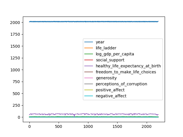
Basic Line Plot
By default, it plots all numeric columns against the index.
df.plot()
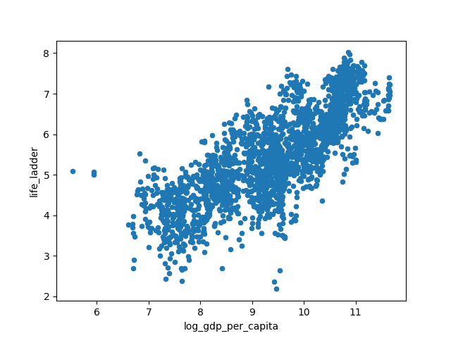
Scatter Plot
Scatter plots are useful for exploring relationships between variables. Here we plot Log GDP per capita vs Life Ladder score.
df.plot(kind='scatter', x='log_gdp_per_capita', y='life_ladder')
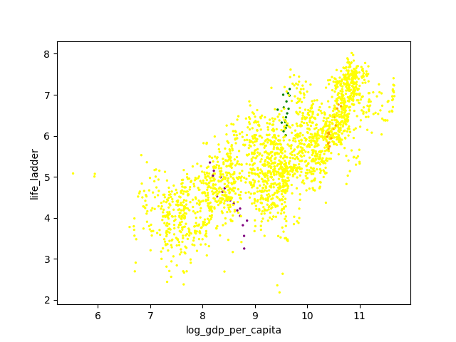
More Customization
You can also use custom colors and sizes:
cmap = {'Brazil': 'Green', 'Slovenia': 'Orange', 'India': 'purple'}
df.plot(
    kind='scatter',
    x='log_gdp_per_capita',
    y='life_ladder',
    c=[cmap.get(c, 'yellow') for c in df.country_name],
    s=2
)
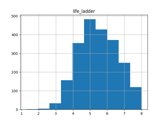
Histogram
To see the distribution of a single column:
df.hist("life_ladder")
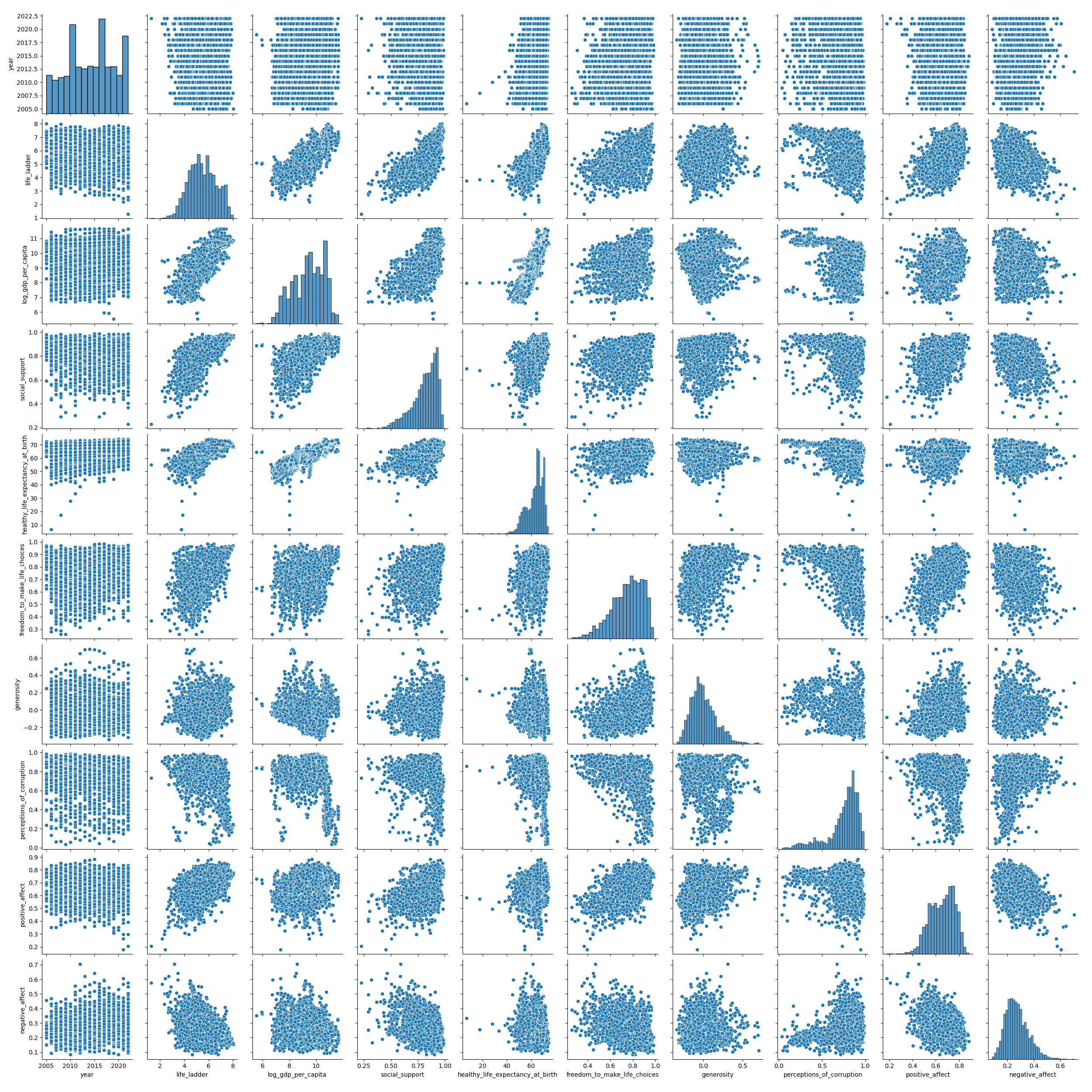
Pair Plot
With this kind of plot, you can see pairwise scatter plots for each pair of columns. On the diagonal (where both columns are the same), you don’t have a scatter plot (which would only show a line), but a histogram showing the distribution of datapoints.
sns.pairplot(df)
6. Operations on Columns
You can easily create new columns from existing ones using arithmetic operations.
# Create a new column as a difference of two others
df["net_affect_difference"] = df["positive_affect"] - df["negative_affect"]
df.head()
Applying Functions
For more advanced operations, use .apply():
# Rescale life_ladder using a lambda function
df['life_ladder_rescaled'] = df['life_ladder'].apply(lambda x: x / 10)

# Apply a custom function
def my_function(x):
    return x * 2

df['my_function'] = df['life_ladder'].apply(my_function)
Congratulations! You’ve completed Pandas 101. You now have the skills to start exploring and manipulating datasets using this powerful library.