Calculus 103: Optimization Using Gradient Descent in Two Variables

In the previous post, we explored optimization for functions of one variable using gradient descent. Now, we will extend this concept to functions of two variables, $f(x, y)$. The principles remain the same: we calculate the gradient (which is now a vector of partial derivatives) and move in the opposite direction to find the minimum.

Navigating optimization landscapes in higher dimensions introduces new challenges, such as saddle points and complex surfaces with multiple local minima. In this post, we will visualize these surfaces and see how gradient descent mimics a ball rolling down a hill.

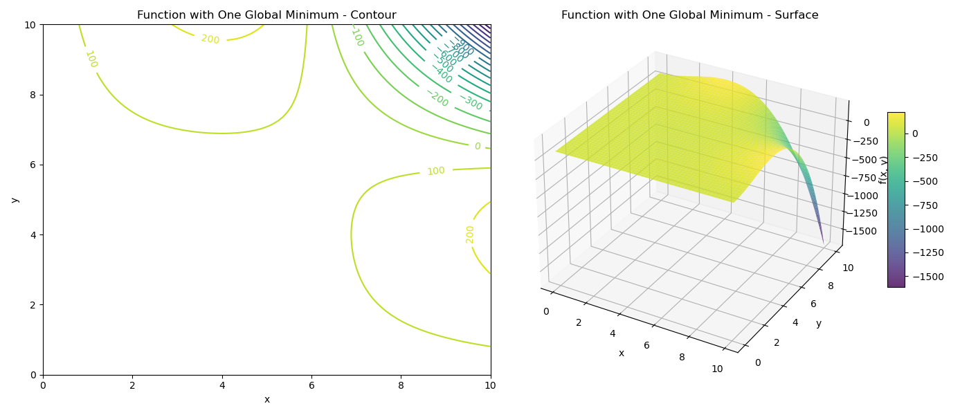
1. Function with One Global Minimum

Let’s start with a function that has a single global minimum. This is the ideal scenario for gradient descent.

Consider the function:

This function, though looking a bit complex, forms a “bowl” shape in a specific region, perfect for demonstrating convergence.

Implementation

First, let’s substitute matplotlib.pyplot and numpy imports.

import numpy as np
import matplotlib.pyplot as plt

We define the function and its partial derivatives, $\frac{\partial f}{\partial x}$ and $\frac{\partial f}{\partial y}$.

def f_example_3(x, y):
    return (85 + 0.1 * (- 1/9 * (x-6) * x**2 * y**3 + 2/3 * (x-6) * x**2 * y**2))

def dfdx_example_3(x, y):
    return 0.1/3 * x * y**2 * (2 - y/3) * (3*x - 12)

def dfdy_example_3(x, y):
    return 0.1/3 * (x-6) * x**2 * y * (4 - y)

Let’s visualize this function using both a contour plot and a 3D surface plot.

Gradient Descent in 2D

The gradient descent update rule for two variables is:

where $\alpha$ is the learning rate.

def gradient_descent_2d(dfdx, dfdy, x, y, learning_rate=0.1, num_iterations=100):
    """
    Performs gradient descent optimization for a 2D function.
    """
    history = [(x, y)]
    for _ in range(num_iterations):
        grad_x = dfdx(x, y)
        grad_y = dfdy(x, y)
        x = x - learning_rate * grad_x
        y = y - learning_rate * grad_y
        history.append((x, y))
    return x, y, history # Return final position and history

For this smooth, bowl-shaped function, gradient descent will reliably converge to the minimum from almost any starting point within the basin of attraction.

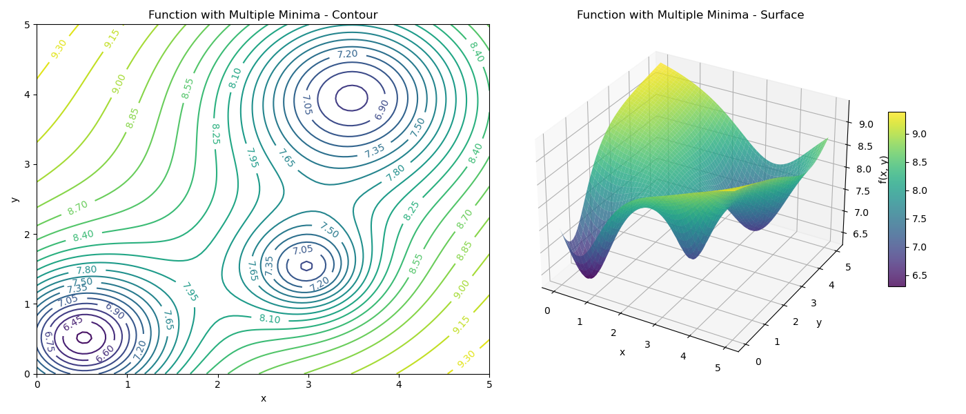
2. Function with Multiple Minima

Real-world optimization problems are rarely as simple as a single bowl. They often have multiple peaks and valleys (local maxima and minima).

Consider this more complex function:

This function has three “holes” or minima of varying depths.

def f_example_4(x, y):
    return -(10/(3+3*(x-.5)**2+3*(y-.5)**2) + \
            2/(1+2*((x-3)**2)+2*(y-1.5)**2) + \
            3/(1+.5*((x-3.5)**2)+0.5*(y-4)**2))+10

# Partial derivatives are calculated using the chain rule (omitted for brevity, see provided code)

Let’s visualize the landscape.

Sensitivity to Initialization

Just like in the 1D case, the starting point determines which minimum the algorithm will find.

• If we start near the deepest hole (global minimum), we naturally slide into it.
• If we start near a shallower hole (local minimum), we get trapped there.
• If we start on a flat region (plateau) or a ridge (saddle point), the gradient might be very small, leading to slow convergence or getting stuck.

Let’s visualize gradient descent paths from varying starting points:

1. Path 1 (Red): Starts near (0.5, 0.5) and converges to the global minimum.
2. Path 2 (Blue): Starts near (3.0, 3.0) and converges to a local minimum.
3. Path 3 (Green): Starts near (3.0, 1.0) and also finds a local minimum.

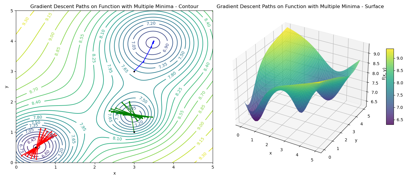
This visually demonstrates that gradient descent is a local optimization algorithm. It finds the nearest minimum, not necessarily the best one.

Conclusion

optimizing functions of two variables allows us to visualize the concepts of gradient descent on a surface. We’ve seen that:

1. For convex-like functions (one global minimum), gradient descent works reliably.
2. For non-convex functions (multiple minima), the initialization point is critical.

In high-dimensional spaces (like training update deep neural networks), these problems mimic what we see in 2D but are even more complex. Techniques like Stochastic Gradient Descent (SGD), Momentum, and Adam are designed to help navigate these tricky landscapes, escaping local minima and saddle points more effectively.