Optimization functions are the core of many machine learning algorithms. To understand how to optimize functions using gradient descent, we’ll start from simple examples: functions of one variable. In this post, we will implement the gradient descent method for functions with single and multiple minima, experiment with the parameters, and visualize the results. This will allow you to understand the advantages and disadvantages of the gradient descent method.
1. Function with One Global Minimum
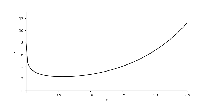
Let’s look at the function $f\left(x\right)=e^x - \log(x)$ (defined for $x>0$). This function has only one minimum point (called a global minimum). However, sometimes that minimum point cannot be found analytically by solving the equation $\frac{df}{dx}=0$. It can be done using a gradient descent method.
To implement gradient descent, you need to start from some initial point $x_0$. Aiming to find a point where the derivative equals zero, you want to move “down the hill”. Calculate the derivative $\frac{df}{dx}(x_0)$ (called a gradient) and step to the next point using the expression:
$$x_1 = x_0 - \alpha \frac{df}{dx}(x_0)$$where $\alpha>0$ is a parameter called a learning rate. Repeat the process iteratively. The number of iterations $n$ is usually also a parameter.
Subtracting $\frac{df}{dx}(x_0)$, you move “down the hill” against the increase of the function — toward the minimum point. So, $\frac{df}{dx}(x_0)$ generally defines the direction of movement. Parameter $\alpha$ serves as a scaling factor.
Implementation
First, let’s load the necessary packages.
import numpy as np
import matplotlib.pyplot as plt

# Magic command to make matplotlib plots interactive if using Jupyter
%matplotlib inline
Now, define the function $f\left(x\right)=e^x - \log(x)$ and its derivative $\frac{df}{dx}\left(x\right)=e^x - \frac{1}{x}$:
def f_example_1(x):
    return np.exp(x) - np.log(x)

def dfdx_example_1(x):
    return np.exp(x) - 1/x
Let’s plot this function to visualize it.
def plot_function(f, x_range, y_range):
    x = np.linspace(x_range[0], x_range[1], 400)
    y = f(x)
    plt.figure(figsize=(8, 6))
    plt.plot(x, y)
    plt.ylim(y_range)
    plt.grid(True)
    plt.xlabel('x')
    plt.ylabel('f(x)')
    plt.title('Function Plot')
    plt.show()

plot_function(f_example_1, [0.001, 2.5], [-0.3, 13])
Gradient descent can be implemented in the following function:
def gradient_descent(dfdx, x, learning_rate=0.1, num_iterations=100):
    """
    Performs gradient descent optimization.

    Arguments:
    dfdx -- function, the derivative of the function to optimize
    x -- float, initial point
    learning_rate -- float, the learning rate (alpha)
    num_iterations -- int, number of iterations

    Returns:
    x -- float, the optimized value after num_iterations
    """
    for iteration in range(num_iterations):
        x = x - learning_rate * dfdx(x)
    return x
Note that there are three parameters in this implementation: num_iterations, learning_rate, and the initial point x. Model parameters for such methods as gradient descent are usually found experimentally. For now, assume we know the parameters that will work.
num_iterations = 25
learning_rate = 0.1
x_initial = 1.6

x_min = gradient_descent(dfdx_example_1, x_initial, learning_rate, num_iterations)
print("Gradient descent result: x_min =", x_min)
Output:
Gradient descent result: x_min = 0.5671434156768685
Analyzing Parameters
The efficiency of gradient descent depends heavily on the choice of parameters.
Learning Rate ($\alpha$):
- If $\alpha$ is too small (e.g.,
0.04with few iterations), the model may not converge to the minimum because the steps are too tiny. - If $\alpha$ is too large (e.g.,
0.5), the method might overshoot and fail to converge, or even diverge. - A moderate value like
0.1or0.3often works well for this smooth function.
- If $\alpha$ is too small (e.g.,
Initial Point ($x_0$):
- Starting closer to the minimum (e.g.,
1.6) helps convergence. - Starting at a very steep part of the function (e.g.,
0.02for this specific function) can cause instability because the gradient is very large, leading to a huge first step that might shoot off to a region where the function is undefined or invalid.
- Starting closer to the minimum (e.g.,
Number of Iterations:
- More iterations generally help convergence but increase computation time.
2. Function with Multiple Minima
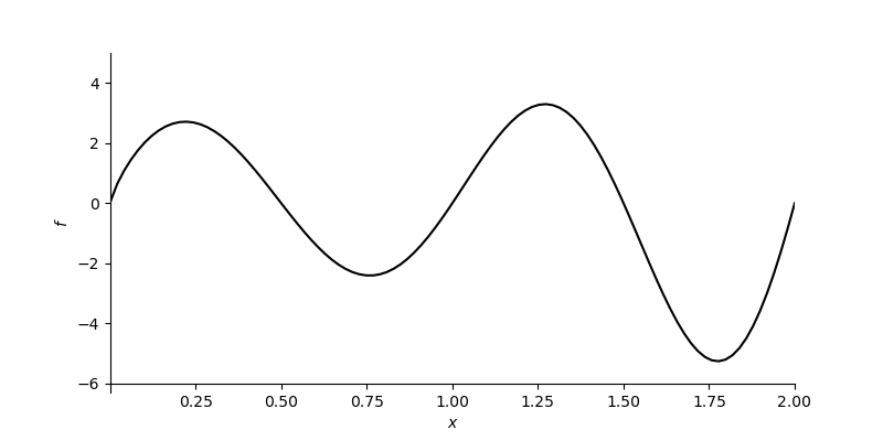
Now let’s look at a slightly more complicated example: a function with multiple minima. This often happens in practice (e.g., in complex loss surfaces for neural networks), where you have local minima and one global minimum.
Consider the function $f(x) = \cos(2x^2) + 0.5x$.
def f_example_2(x):
    return np.cos(2 * x**2) + 0.5 * x

def dfdx_example_2(x):
    return -np.sin(2 * x**2) * 4 * x + 0.5
Let’s plot it:
plot_function(f_example_2, [0, 2.5], [-2, 2])
Now let’s run gradient descent with the same learning rate and iterations but different starting points.
learning_rate = 0.005
num_iterations = 35

# Case 1: Start at 1.3
x_initial_1 = 1.3
min_1 = gradient_descent(dfdx_example_2, x_initial_1, learning_rate, num_iterations)
print(f"Start at {x_initial_1}: Minimum found at {min_1:.4f}")

# Case 2: Start at 0.25
x_initial_2 = 0.25
min_2 = gradient_descent(dfdx_example_2, x_initial_2, learning_rate, num_iterations)
print(f"Start at {x_initial_2}: Minimum found at {min_2:.4f}")
Output:
Start at 1.3: Minimum found at 1.7752
Start at 0.25: Minimum found at 0.7586
Observations
The results will likely be different.
- In one case, the algorithm might slide down to the global minimum.
- In the other, it might get “stuck” in a local minimum.
This illustrates a key limitation of standard gradient descent: it is sensitive to initialization. If you start in the “basin” of a local minimum, you will converge to that local minimum, not necessarily the global one.
Conclusion
Gradient descent is a robust and widely used optimization method. It allows you to optimize a function with relatively simple calculations. However, it has drawbacks:
- Sensitivity to Parameters: The learning rate must be chosen carefully.
- Initialization: For non-convex functions (those with multiple minima), the starting point determines which minimum you reach.
In future posts, we will explore methods to mitigate these issues, such as using momentum or adaptive learning rates.