Calculus 101: Differentiation in Python

Derivatives are fundamental to calculus and essential for machine learning applications. In this post, we explore three powerful methods for computing derivatives in Python: symbolic differentiation with SymPy, numerical differentiation with NumPy, and automatic differentiation with JAX.

Why Differentiation Matters

In real-world applications, functions can be quite complex, making analytical differentiation impractical. Python provides several tools to compute derivatives automatically, each with different trade-offs in terms of accuracy, speed, and ease of use.

Functions in Python

Let’s start with a simple reminder of how to define functions in Python. Consider the function $f(x) = x^2$:

def f(x):
    return x**2

print(f(3))  # Output: 9

The derivative of this function is $f'(x) = 2x$:

def dfdx(x):
    return 2*x

print(dfdx(3))  # Output: 6

We can apply these functions to NumPy arrays:

import numpy as np

x_array = np.array([1, 2, 3])
print("x:", x_array)
print("f(x) = x**2:", f(x_array))  # [1 4 9]
print("f'(x) = 2x:", dfdx(x_array))  # [2 4 6]

Here’s what these functions look like when plotted together:

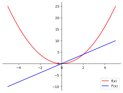
The red curve shows our function $f(x) = x^2$, while the blue line shows its derivative $f'(x) = 2x$. Notice how the derivative tells us the slope of the function at each point.

Symbolic Differentiation with SymPy

Symbolic computation deals with mathematical objects represented exactly, not approximately. For differentiation, this means the output is similar to computing derivatives by hand using calculus rules.

Introduction to SymPy

SymPy is a Python library for symbolic mathematics. Unlike numerical computation that gives approximate results like $\sqrt{18} \approx 4.242640687$, SymPy simplifies expressions exactly:

from sympy import *

sqrt(18)  # Output: 3*sqrt(2)

To define symbolic variables and expressions:

x, y = symbols('x y')
expr = 2 * x**2 - x * y
expr  # Output: 2*x**2 - x*y

You can manipulate expressions symbolically:

expand(expr * x + x**4)  # Expand the expression
factor(expr)  #  Factorize the expression

Computing Derivatives

Computing derivatives with SymPy is straightforward:

diff(x**3, x)  # Output: 3*x**2

SymPy handles complex functions using the chain rule automatically:

from sympy import exp, sin, cos

dfdx_composed = diff(exp(-2*x) + 3*sin(3*x), x)
# Output: 9*cos(3*x) - 2*exp(-2*x)

To use symbolic derivatives with NumPy arrays, convert them using lambdify:

from sympy.utilities.lambdify import lambdify

f_symb = x ** 2
dfdx_symb = diff(f_symb, x)
dfdx_symb_numpy = lambdify(x, dfdx_symb, 'numpy')

x_array = np.array([1, 2, 3])
dfdx_symb_numpy(x_array)  # Output: [2 4 6]

Here’s the symbolic derivative plotted alongside the original function:

This plot demonstrates how SymPy can compute exact derivatives symbolically, then convert them to NumPy-compatible functions for plotting and numerical evaluation.

Limitations of Symbolic Differentiation

While powerful, symbolic differentiation has limitations:

1. Discontinuities: Functions with “jumps” in derivatives (like the absolute value function) produce complicated, sometimes unevaluable expressions.

2. Expression Swell: Complex functions can produce very complicated derivative expressions that are slow to compute.

For the absolute value function $|x|$, SymPy produces a complex expression that can’t be easily evaluated at all points.

Numerical Differentiation with NumPy

Numerical differentiation uses the fundamental definition of a derivative as a limit:

where $\Delta x$ is sufficiently small.

Using np.gradient()

NumPy’s gradient function approximates derivatives numerically:

x_array = np.linspace(-5, 5, 100)
dfdx_numerical = np.gradient(f(x_array), x_array)

Here’s how the numerical approximation compares to the exact derivative:

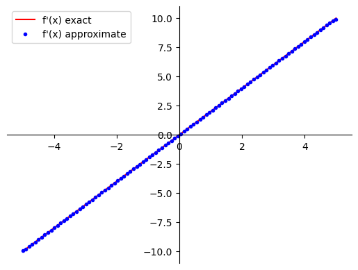
The solid blue line is the exact derivative, while the dots are the numerical approximation from np.gradient(). The results are remarkably accurate!

For more complex functions, numerical differentiation still performs well:

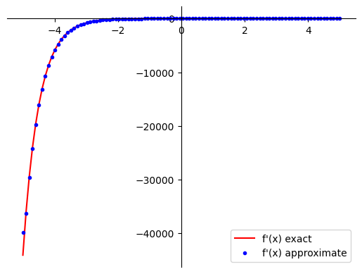
Even for $f(x) = e^{-2x} + 3\sin(3x)$, the numerical method (blue dots) closely matches the exact derivative (blue line).

The results are impressively accurate for most functions. The key advantage is that it doesn’t matter how the function was calculated - only the final values matter!

Limitations of Numerical Differentiation

1. Approximation Errors: Results are not exact, though usually accurate enough for machine learning.

2. Discontinuities: Like symbolic differentiation, numerical methods struggle at points where derivatives have “jumps.”

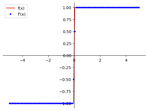
This plot shows the derivative of $|x|$. The exact derivative should be 1 for $x > 0$ and -1 for $x < 0$, but the numerical method gives incorrect values like 0.5 and -0.5 near the discontinuity at $x=0$.

3. Computational Cost: The biggest problem is speed. Every derivative requires a full function evaluation, which becomes expensive with hundreds of parameters in machine learning models.

Automatic Differentiation with JAX

Automatic differentiation (autodiff) combines the best of both worlds. It breaks down functions into elementary operations, builds a computational graph, and uses the chain rule to compute exact derivatives efficiently.

Introduction to JAX

JAX is a modern library that combines automatic differentiation (Autograd) with accelerated linear algebra (XLA) for parallel computing:

from jax import grad, vmap
import jax.numpy as jnp

JAX arrays work similarly to NumPy arrays but support automatic differentiation and can run on GPUs.

Computing Derivatives

The grad() function computes derivatives automatically:

# Define a function
def f(x):
    return x ** 2

# Get the gradient function
dfdx_auto = grad(f)

# Evaluate at a point
dfdx_auto(3.0)  # Output: 6.0

For arrays, use vmap() to vectorize:

dfdx_auto_vec = vmap(dfdx_auto)
x_array = jnp.linspace(-5, 5, 100)
dfdx_auto_vec(x_array)

Here’s the result of JAX automatic differentiation:

JAX computes the derivative using automatic differentiation, which is both exact (like symbolic) and fast (like numerical for simple cases). The plot shows how grad() and vmap() work together to compute derivatives across arrays efficiently.

JAX handles complex compositions automatically:

def f_composed(x):
    return jnp.exp(-2*x) + 3*jnp.sin(3*x)

dfdx_composed_auto = grad(f_composed)

Why Automatic Differentiation?

Autodiff is the standard in modern machine learning frameworks because:

1. Exact Derivatives: Unlike numerical methods, it computes exact derivatives (up to floating-point precision)
2. Fast Computation: The computational graph is built once and reused
3. Handles Complexity: Works seamlessly with complex functions and compositions
4. GPU Support: JAX can leverage GPU acceleration for massive speedups

Performance Comparison

When comparing the three methods on complex functions with many parameters:

• Symbolic: Slowest due to expression complexity and repeated symbolic manipulation
• Numerical: Medium to slow, requires repeated function evaluations
• Automatic: Fastest, especially with GPU support, as the computation graph is built once

For machine learning applications with hundreds or thousands of parameters, automatic differentiation is typically 10-100x faster than the alternatives.

Summary

Understanding differentiation in Python comes down to choosing the right tool:

• SymPy (Symbolic): Best for exact analytical results and symbolic manipulation; limited by expression complexity

• NumPy (Numerical): Simple to implement and function-agnostic; limited by approximation errors and computational cost

• JAX (Automatic): The modern standard for machine learning; combines exactness with computational efficiency

For most machine learning applications, automatic differentiation with JAX provides the best balance of accuracy, speed, and ease of use.