Stan 101 with Logistic Regression

Stan is where we onboard teammates to Bayesian workflows. A logistic regression is the gentlest way to see how Stan’s modeling language, inference engine, and diagnostics line up, so this post walks through the full pipeline end-to-end.

Logistic regression in equations

For observation $n = 1, \ldots, N$ with predictors $x_n \in \mathbb{R}^K$ and binary outcome $y_n \in {0, 1}$, the logistic regression model is

$$ \begin{aligned} y_n &\sim \operatorname{Bernoulli}(\theta_n), \ \theta_n &= \operatorname{logit}^{-1}(\eta_n), \ \eta_n &= \alpha + x_n^\top \beta, \end{aligned} $$

where $\alpha$ is the intercept, $\beta \in \mathbb{R}^K$ are slope coefficients, and $\operatorname{logit}^{-1}(z) = \frac{1}{1 + e^{-z}}$. In vector form, with design matrix $X \in \mathbb{R}^{N \times K}$, the linear predictor is $\eta = \alpha \mathbf{1}_N + X \beta$. Here $\mathbf{1}_N$ represents an $N$-dimensional column vector of ones, so $\alpha \mathbf{1}_N$ is simply the intercept repeated for every observation; adding it to $X \beta$ shifts each linear predictor by the same baseline amount. The Stan program below encodes this model along with weakly informative priors on $\alpha$ and $\beta$.

Why Stan for discrete outcomes

• Express the likelihood and priors directly in Stan’s modeling language without wrestling with black-box abstractions.
• Leverage Hamiltonian Monte Carlo (HMC) to explore posteriors that simple Metropolis samplers struggle with.
• Inspect diagnostics (divergences, effective sample sizes, R-hat) that ship by default with every fit.
• Reuse the same Stan program across R, Python, or the command-line interface.

1. Scaffold a minimal Stan project

We’ll use cmdstanpy, which gives Python bindings to the CmdStan interface. Once you install CmdStan (cmdstanpy.install_cmdstan()) the wrapper takes care of compilation and sampling.

from cmdstanpy import CmdStanModel
import pandas as pd
import numpy as np

# Toy admissions dataset: GPA + GRE scores predicting acceptance
students = pd.DataFrame(
    {
        "gpa": [2.5, 3.2, 3.8, 2.9, 3.6, 3.1, 2.7, 3.9, 3.4, 2.8],
        "gre": [480, 600, 720, 520, 700, 640, 500, 760, 660, 540],
        "admit": [0, 0, 1, 0, 1, 1, 0, 1, 1, 0],
    }
)
students["gre_std"] = (students["gre"] - students["gre"].mean()) / students["gre"].std()
students["gpa_std"] = (students["gpa"] - students["gpa"].mean()) / students["gpa"].std()

Standardizing predictors keeps the sampler happy because the coefficients live on comparable scales.

2. Assemble data for Stan

Stan consumes a dictionary of primitives. Split out the design matrix and response, then feed them to the model.

X = students[["gre_std", "gpa_std"]].to_numpy()
stan_data = {
    "N": students.shape[0],
    "K": X.shape[1],
    "X": X,
    "y": students["admit"].to_numpy(),
}

3. Write the Stan program

The Stan file defines the generative story: priors on the intercept and weights, a Bernoulli likelihood with logit link, and a generated quantities block for pointwise log-likelihood (useful for LOO or WAIC later).

data {
  int<lower=0> N;
  int<lower=1> K;
  matrix[N, K] X;
  array[N] int<lower=0, upper=1> y;
}
parameters {
  real alpha;
  vector[K] beta;
}
model {
  alpha ~ normal(0, 5);
  beta ~ normal(0, 2.5);
  y ~ bernoulli_logit(alpha + X * beta);
}
generated quantities {
  array[N] real log_lik;
  array[N] int<lower=0, upper=1> y_hat;
  for (n in 1:N) {
    real eta = alpha + X[n] * beta;
    log_lik[n] = bernoulli_logit_lpmf(y[n] | eta);
    y_hat[n] = bernoulli_logit_rng(eta);
  }
}

Keep the file as models/logistic_regression.stan (or similar) inside your project.

4. Compile and sample

With CmdStan installed, compilation translates the Stan program into optimized C++. Sampling launches four HMC chains by default.

model = CmdStanModel(stan_file="models/logistic_regression.stan")
fit = model.sample(
    data=stan_data,
    iter_warmup=1000,
    iter_sampling=1000,
    chains=4,
    seed=20251030,
)
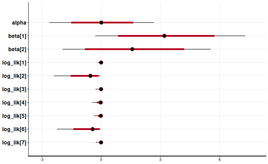
fit.summary()

You’ll see posterior estimates for the intercept (alpha) and standardized coefficients (beta[1] for GRE, beta[2] for GPA), plus diagnostics like R_hat, bulk/tail ess, and divergence counts.

5. Diagnose and interpret

Stan surfaces rich diagnostics—treat them as required reading, not optional.

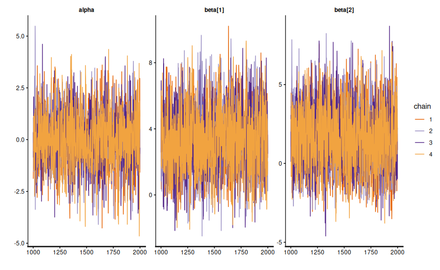
• fit.diagnose() flags divergences or treedepth saturations that mean the sampler struggled; address them with better priors or reparameterization.
• Trace plots (fit.draws()) reassure you that chains mix and explore the posterior rather than sticking to a single mode.

• Posterior predictive checks compare y_hat draws to the observed admissions. If the simulated acceptance rates miss the observed rate completely, revisit the model.
• Leave-one-out cross-validation becomes trivial with the log_lik vector: arviz.loo(fit.to_inference_data()) ranks competing specifications.

6. Extend the template

Logistic regression is just the opening move. Stan makes it straightforward to:

• Add hierarchical structure by letting intercepts or slopes vary by department (alpha[dept] ~ normal(mu_alpha, sigma_alpha)).
• Swap in regularizing priors (e.g., beta ~ normal(0, 1) or horseshoe priors) when predictors explode.
• Incorporate interaction terms or nonlinear basis expansions before handing data to Stan.
• Move to ordered logistic or multinomial likelihoods when the response has more than two categories.

Each extension reuses the same data → model → sampling pipeline, so the initial investment pays off quickly.

7. Takeaways

• A small, fully worked example makes Stan approachable before tackling hierarchical or time-series models.
• Standardized predictors, explicit priors, and posterior predictive checks keep logistic regression fits stable.
• CmdStanPy bridges Python workflows with Stan’s compiled performance, while sharing Stan programs across teams.
• Diagnostics (fit.diagnose(), R_hat, effective sample sizes) are first-class signals that the posterior is trustworthy.
• The same pattern scales to richer discrete-outcome models—logistic regression is simply the friendliest starting point.