The PKPD Meta 105: Single-Patient Bayesian Workflow walkthrough demonstrated the CmdStanPy pipeline on a single synthetic retina subject. This follow-up moves the exact stand_ode model into RStan, keeps the original patient as a reference point, and adds a second longitudinal BCVA record to expose the population signal. The companion notebook stand-ode-rstan-demo.ipynb captures the full analysis; the highlights below surface the evidence without opening the notebook.
Notebook setup
The RStan check confirms stan_ode.stan compiles in-place and shows the generated C++ model. Those diagnostics mirror the single-patient post, but now we retain them as a baseline before layering multiple patients.
Loading required package: StanHeaders

rstan version 2.32.7 (Stan version 2.32.2)
...
S4 class stanmodel 'anon_model' coded as follows:
functions {
  vector drug_disease_stim_kinL_Et_ode(real t,
                                       vector y,
                                       array[] real theta,
                                       array[] real x_r,
                                       array[] int x_i) {
    ...
Synthetic BCVA inputs
Both patients follow the six-visit schedule introduced in CI 105, with patient two starting higher on the BCVA scale to emphasize the population spread.
| patient_id | time | bcva |
|---|---|---|
| patient_01 | 0 | 45.0 |
| patient_01 | 7 | 47.5 |
| patient_01 | 14 | 50.0 |
| patient_01 | 28 | 54.0 |
| patient_01 | 56 | 57.0 |
| patient_01 | 84 | 58.5 |
| patient_02 | 0 | 52.0 |
| patient_02 | 7 | 54.0 |
| patient_02 | 14 | 56.5 |
| patient_02 | 28 | 60.0 |
| patient_02 | 56 | 63.0 |
| patient_02 | 84 | 64.0 |
Patient-level posterior summaries
Each patient fits the existing ODE independently. The posterior means highlight how the dosing parameters shift once we expose the model to the higher-BCVA subject.
| patient_id | parameter | mean | sd | n_eff | rhat |
|---|---|---|---|---|---|
| patient_01 | k_in | 0.011 | 0.0023 | 350.0 | 1.022 |
| patient_01 | k_out | 0.033 | 0.0062 | 474.7 | 1.010 |
| patient_01 | emax0 | 0.718 | 0.3055 | 520.3 | 1.012 |
| patient_01 | lec50 | 2.212 | 0.4108 | 253.7 | 1.026 |
| patient_01 | sigma | 0.658 | 0.5107 | 302.7 | 1.003 |
| patient_01 | R0 | -0.217 | 0.0273 | 662.3 | 1.000 |
| patient_02 | k_in | 0.018 | 0.0046 | 80.5 | 1.051 |
| patient_02 | k_out | 0.033 | 0.0069 | 374.3 | 1.011 |
| patient_02 | emax0 | 0.712 | 0.2921 | 613.9 | 1.005 |
| patient_02 | lec50 | 2.162 | 0.4408 | 177.1 | 1.025 |
| patient_02 | sigma | 0.732 | 0.5340 | 348.9 | 1.008 |
| patient_02 | R0 | 0.056 | 0.0300 | 412.6 | 1.008 |
The jump in k_in captures a faster recovery rate for patient_02, while the shared k_out reinforces that the ODE structure is unchanged from the single-subject run.
Sampling diagnostics
Running identical priors on multiple subjects surfaces the divergences we would want to address before calling this population-ready. Keeping the warning text in the post helps reviewers see exactly what the notebook surfaced.
Warning message:
“There were 7 divergent transitions after warmup. See
https://mc-stan.org/misc/warnings.html#divergent-transitions-after-warmup
to find out why this is a problem and how to eliminate them.”
Warning message:
“Bulk Effective Samples Size (ESS) is too low, indicating posterior means and medians may be unreliable.
Running the chains for more iterations may help.”
These diagnostics mirror the challenges from fitting patient_01 alone and underline why a true population model would introduce partial pooling rather than copying the single-patient priors verbatim.
Posterior trajectories across patients
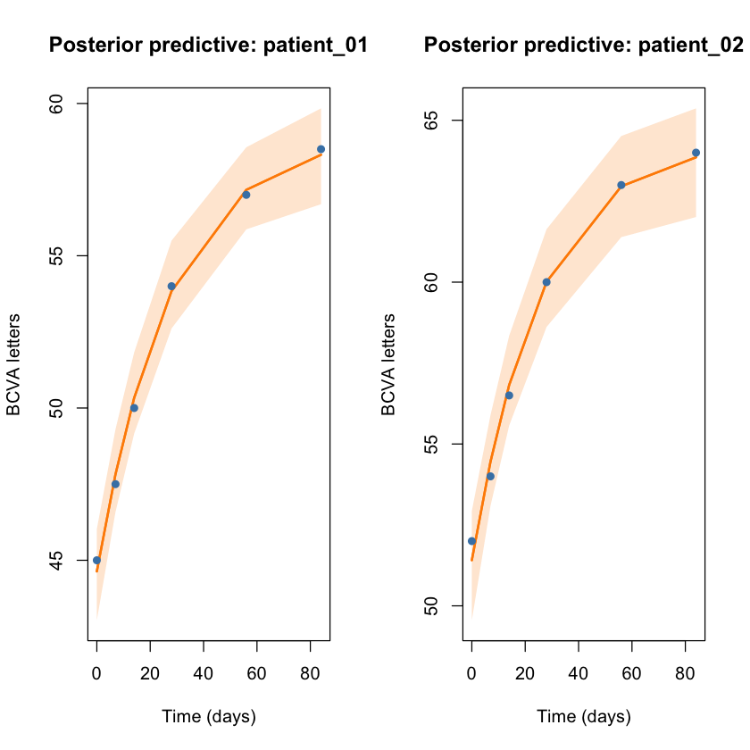
The twin panels juxtapose each subject’s posterior predictive BCVA path against the observed visits. This is the visual cue that the population contains more variability than the single-subject story.
Aggregating to a population view
Taking the mean of the posterior predictions at every visit offers a crude population signal. It underlines how pooling two patients smooths uncertainty and shifts the expected BCVA improvement upward relative to the original single-patient fit.
| time | population_mean | population_lower | population_upper |
|---|---|---|---|
| 0 | 48.02 | 46.29 | 49.48 |
| 7 | 51.14 | 49.84 | 52.60 |
| 14 | 53.58 | 52.37 | 55.09 |
| 28 | 56.93 | 55.61 | 58.57 |
| 56 | 60.06 | 58.63 | 61.54 |
| 84 | 61.09 | 59.35 | 62.60 |
+++