PKPD 104: Turnover Models for Indirect Response

PKPD 101 established the concentration-time backbone, PKPD 102 reviewed direct-effect relationships, and PKPD 103 introduced effect compartments for biophase lags. Turnover models cover the remaining ground: biomarkers or clinical endpoints governed by slow biosynthesis and degradation. When the drug perturbs either production or loss, the effect evolves according to the kinetics of that turnover pool rather than plasma concentration alone.

When an indirect response model is the right tool

• Baseline measurements follow a homeostatic balance between synthesis and loss (e.g., endogenous metabolites, cytokines, clotting factors).
• Drug effects persist long after concentrations fade because the pool must regenerate or decay.
• Dose escalation shows delay to both onset and offset, even after accounting for distribution lags.
• Placebo responses already exhibit gradual drifts, hinting at turnover dynamics that the drug magnifies or suppresses.
• Sampling near the pharmacokinetic peak shows little change, but later time points diverge markedly from baseline.

These signatures flag that the target variable is dynamically buffered. Modeling the feedback via synthesis ($k_\text{in}$) and loss ($k_\text{out}$) rates captures both timing and magnitude.

Anatomy of turnover models

The canonical indirect response structure tracks a turnover state $R(t)$ that satisfies

where $k_\text{in}$ is the zero-order production rate and $k_\text{out}$ is the first-order loss rate that defines the baseline $R_0 = k_\text{in}/k_\text{out}$. Drug concentration modulates either production or loss through stimulation ($S > 0$) or inhibition ($S < 0$).

Four archetypes cover most applications:

• Model I (stimulate production): $S_\text{in}(C) = S_\text{max} \frac{C^\gamma}{SC_{50}^\gamma + C^\gamma}$; $S_\text{out}(C) = 0$.
• Model II (inhibit production): $S_\text{in}(C) = -I_\text{max} \frac{C^\gamma}{IC_{50}^\gamma + C^\gamma}$.
• Model III (stimulate loss): $S_\text{out}(C) = S_\text{max} \frac{C^\gamma}{SC_{50}^\gamma + C^\gamma}$.
• Model IV (inhibit loss): $S_\text{out}(C) = -I_\text{max} \frac{C^\gamma}{IC_{50}^\gamma + C^\gamma}$.

Pick the variant that matches the biology: chronotropic drugs often stimulate loss (Model III) of heart-rate control, while anti-inflammatory agents suppress cytokine production (Model II).

Parameter intuition and practical estimation

• $k_\text{out}$ sets the recovery half-life $t_{1/2} = \ln(2)/k_\text{out}$; it controls how long the effect lingers after exposure dissipates.
• $k_\text{in}$ is best inferred from baseline variance—treat $R_0$ as a direct observation and back-calculate $k_\text{in} = k_\text{out} R_0$.
• Stimulation/inhibition maxima ($S_\text{max}$ or $I_\text{max}$) capture fractional changes in production or loss. Constrain them to the plausible biochemical range to avoid overfitting rebounds.
• Potency parameters ($SC_{50}$ or $IC_{50}$) are often poorly informed without late-time sampling; anchor them with priors, literature, or rich design.
• Residual unexplained variability should be evaluated on both the raw scale and turnover state to spot mis-specified baselines or drift.

Worked example: corticosteroid suppression of cortisol

High-dose corticosteroids suppress adrenocorticotropic hormone, thus reducing cortisol production (Model II). A simplified once-daily oral regimen is:

With $k_\text{out}$ corresponding to an 8-hour cortisol half-life, the model captures the observed nadir several hours post-dose and the slow overnight recovery.

Simulating a turnover system

import numpy as np
from scipy.integrate import solve_ivp

CL, V = 12.0, 40.0          # L/h, L
k_in = 50.0                 # nmol/L/h
k_out = np.log(2) / 8.0     # h^-1
Imax, IC50 = 0.9, 20.0      # unitless, nmol/L
dose = 50.0                 # mg
F = 0.8                     # bioavailability

def rhs(t, y):
    Cp, R = y
    dCp = -(CL / V) * Cp
    inhib = Imax * Cp / (IC50 + Cp)
    dR = k_in * (1.0 - inhib) - k_out * R
    return [dCp, dR]

C0 = (F * dose) / V
sol = solve_ivp(rhs, [0.0, 48.0], [C0, k_in / k_out], dense_output=True)
time = np.linspace(0.0, 48.0, 200)
Cp, cortisol = sol.sol(time)

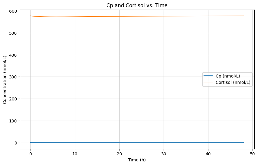
This script integrates turnover dynamics over two days after a single oral dose. The cortisol trajectory shows a delayed nadir and gradual recovery consistent with an inhibited-production mechanism.

The simulated plasma and biomarker curves emphasize how the pharmacodynamic nadir trails the concentration peak and how recovery is governed by $k_\text{out}$ rather than drug clearance.

nmol/L denotes nanomoles per liter, the molar concentration unit used for both $C_p$ and cortisol in this example.

Diagnostics and model qualification

• Plot $R(t)$ and the observed biomarker together; mismatched recovery indicates incorrect $k_\text{out}$.
• Compare concentration-effect loops against turnover-adjusted predictions; indirect response models should straighten loops much like effect compartments do.
• Visual predictive checks on both baseline and post-dose intervals flag whether production and loss are balanced.
• Condition number diagnostics help confirm that $S_\text{max}$ and $IC_{50}$ are estimable; consider fixing one if the design lacks late-time data.
• Evaluate placebo fits with the same $k_\text{out}$ to ensure the turnover mechanism captures natural history.

Communicating the clinical implications

• Translate $k_\text{out}$ into recovery times so clinicians know when to redose or schedule monitoring.
• Highlight whether the drug alters production or loss; this informs combination strategies (e.g., stacking production inhibitors can exaggerate nadirs).
• Document any rebound predictions if $S_\text{max}$ or $I_\text{max}$ exceeds unity—operations teams need to manage overshoot risk.
• Summarize covariate effects on turnover parameters separately from potency terms to clarify sources of variability.

References

• Dayneka NL, Garg V, Jusko WJ. J Pharmacokinet Biopharm. 1993;21:457–478.
• Sharma A, Jusko WJ. Clin Pharmacokinet. 1998;35:347–363.
• Mager DE, Jusko WJ. J Pharm Sci. 2008;97:2221–2237.