PKPD 101 built the concentration-time intuition you need to trust exposure predictions, while PKPD 102 stayed in the realm of direct-response models. This installment tackles the opposite scenario: you observe a clear delay between drug concentration and effect that cannot be captured with instantaneous transduction. We will stay focused on effect compartment models—how to recognize when you need them, estimate their parameters, and interpret what they say about equilibration at the site of action.
Recognizing when an effect compartment is needed
- Effect-versus-concentration plots show counterclockwise loops (hysteresis) that collapse only after adding a lag or effect compartment.
- Onset of effect is slower than distribution half-life, while offset is also delayed despite rapid clearance.
- Clinical intuition points to receptors embedded in tissues with slower equilibration than plasma (e.g., central nervous system, biophase fluids).
- Covariates that plausibly alter biophase access (perfusion, transporter expression, swelling) shift the entire time course, not just magnitude.
These signatures tell you that the system cannot react instantaneously to concentration changes. Delaying concentration via an effect compartment keeps the pharmacodynamic equation familiar while honoring the observed hysteresis.
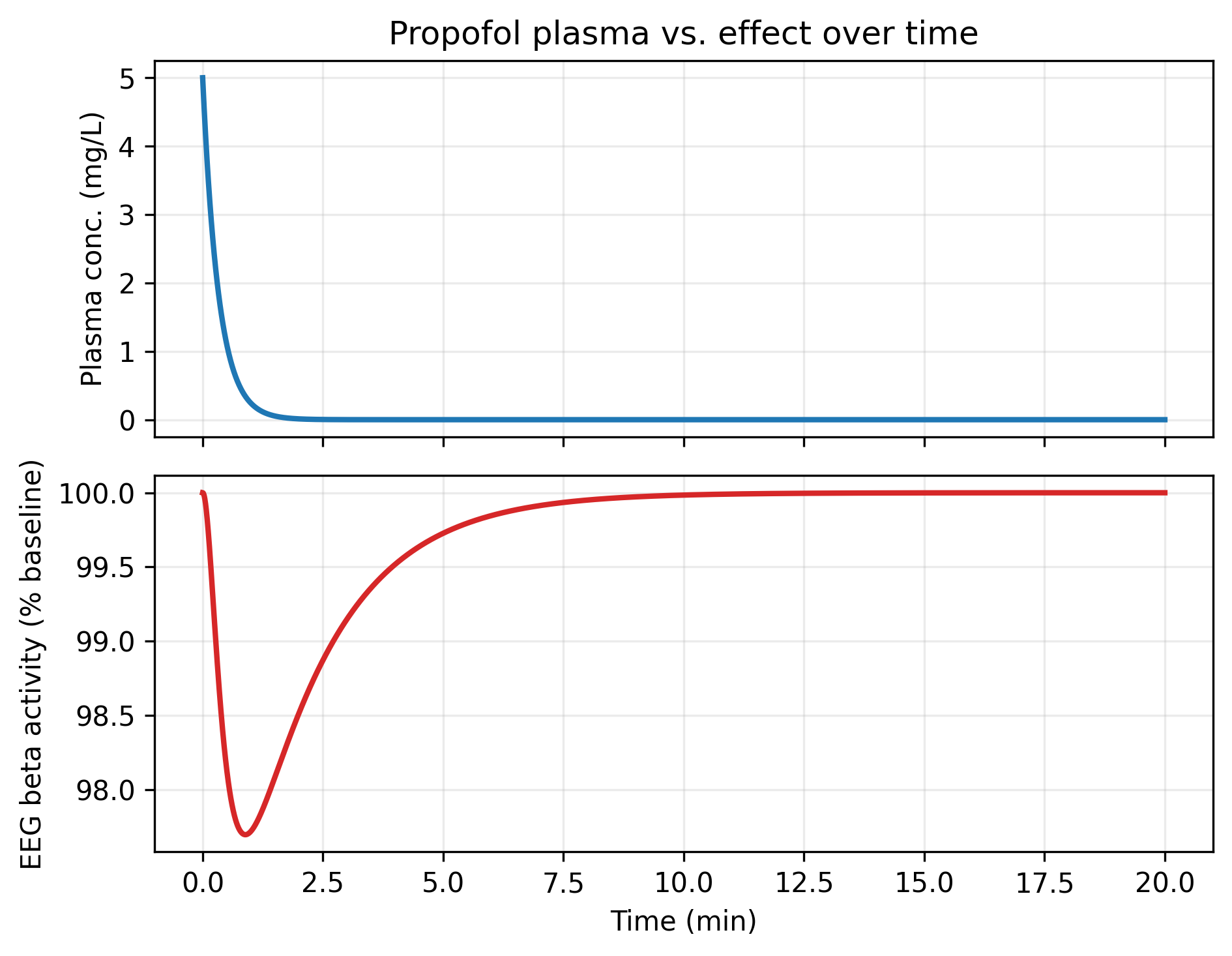
Figure: Plasma concentration (top) decays faster than EEG suppression (bottom), so effect lags exposure. Plotting these traces against each other generates the counterclockwise hysteresis loop characteristic of effect-compartment behavior.
Effect compartment essentials
An effect compartment captures biophase equilibration when receptors sit in a tissue compartment that equilibrates more slowly than plasma. The standard structure is
$$ \frac{dC_e}{dt} = k_{e0} \left(C_p(t) - C_e(t)\right), $$where $C_p$ is the predicted plasma concentration, $C_e$ is the effect-site concentration, and $k_{e0}$ is the first-order equilibration rate. The pharmacodynamic model is then written in terms of $C_e$:
$$ E(t) = E_0 \pm \frac{E_{\max} \, C_e(t)^\gamma}{EC_{50}^\gamma + C_e(t)^\gamma}. $$Parameter intuition and estimation tips
- Small $k_{e0}$ values produce large lags and hysteresis; $t_{1/2,e0} = \ln(2)/k_{e0}$ is a handy descriptor to communicate.
- The slope of the concentration–effect loop near peak effect shrinks as $k_{e0}$ decreases; look for sampling around $t_{1/2,e0}$ to identify it.
- Use observed effect-time data to initialize $k_{e0}$: the delay between $C_\text{max}$ and $E_\text{max}$ is roughly $3$–$4$ half-lives of the effect compartment.
- When fitting nonlinear mixed effects models, estimate $k_{e0}$ before reintroducing $E_{\max}$ variability—their correlation can otherwise stall convergence.
- Link models can connect $C_e$ to intermediate transduction states when the ultimate effect is categorical or composite (e.g., sedation scores).
Worked example: propofol EEG suppression
Propofol produces rapid plasma decay yet a lag in electroencephalogram (EEG) suppression, making it a classic effect-compartment problem. A simplified bolus model is:
$$ \begin{aligned} \frac{dC_p}{dt} &= -\frac{CL}{V} C_p \\ \frac{dC_e}{dt} &= k_{e0} (C_p - C_e) \\ E(t) &= E_0 - \frac{E_{\max} \, C_e(t)^\gamma}{EC_{50}^\gamma + C_e(t)^\gamma} \end{aligned} $$where $E(t)$ is the fraction of baseline beta activity in the EEG. Published analyses (Sheiner & Stanski, Anesthesiology. 1984;60:217–228) report $k_{e0}$ around $0.26 \ \text{min}^{-1}$ for propofol.
Simulating the effect-compartment model
import numpy as np
from scipy.integrate import solve_ivp

CL, V = 90.0, 30.0            # L/min, L
ke0 = 0.26                    # min^-1
E0, Emax = 100.0, 90.0        # baseline %, maximal drop %
EC50, gamma = 1.8, 2.2        # mg/L, Hill coefficient
dose = 150.0                  # mg IV bolus

def rhs(t, y):
    Cp, Ce = y
    dCp = -(CL / V) * Cp
    dCe = ke0 * (Cp - Ce)
    return [dCp, dCe]

C0 = dose / V
sol = solve_ivp(rhs, [0, 20], [C0, 0.0], dense_output=True)
time = np.linspace(0, 20, 200)
Cp, Ce = sol.sol(time)
effect = E0 - Emax * (Ce**gamma) / (EC50**gamma + Ce**gamma)
This script integrates joint PK and effect-compartment equations through 20 minutes. The effect trace shows maximal EEG suppression several minutes after plasma peaks and a slower recovery—behavior impossible to match with a direct-response model.
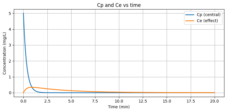
Figure: Solving the coupled PK and effect compartments shows the lagging effect-site concentration that drives delayed onset.
Diagnostics for effect-compartment models
- Plot effect versus $C_p$ and versus $C_e$; only the latter should collapse hysteresis if the effect compartment is appropriate.
- Check conditional weighted residuals against time and $C_e$; structure in residuals often signals mis-specified $k_{e0}$.
- Run visual predictive checks on both effect-time profiles and effect-versus-$C_p$ loops; the VPC for the loop quickly reveals whether hysteresis is captured.
- Profile likelihood or bootstrap $k_{e0}$ alongside potency terms to quantify the strong correlation typically observed.
Communicating model implications
- Translate $k_{e0}$ into a clinically meaningful equilibration half-life and compare against onset/offset expectations.
- Clarify how delayed onset informs titration (e.g., wait two $t_{1/2,e0}$ before adjusting infusions).
- Document whether covariates shift $k_{e0}$ or pharmacodynamic potency—implementation teams need to know if delays or sensitivity drive inter-patient differences.
References
- Sheiner LB, Stanski DR, Vozeh S, Miller RD, Ham J. Anesthesiology. 1979;50:1–12.
- Sheiner LB, Stanski DR. Anesthesiology. 1984;60:217–228.
- Schnider TW, Minto CF, et al. Anesthesiology. 1998;88:1170–1182.