In PKPD 101 we built intuition for concentration-time profiles. This follow-up stays strictly on the direct-response side of pharmacodynamics: situations where the measured effect tracks plasma concentrations closely enough that no effect compartment or turnover structure is needed. You will see how to recognize the pattern, select the right structural model, and verify the fit with published clinical datasets.
When a direct-response model fits
- Concentration and effect are recorded on matching timescales (seconds to minutes for IV drugs—intravenous administration via vein, minutes to hours for oral) and peak together.
- Observed effect-time profiles lack pronounced loops when plotted against concentration—little to no hysteresis.
- The biomarker or clinical endpoint responds faster than drug distribution; no biological turnover pool is obviously rate-limiting.
- Repeated dosing shows immediate reversibility once plasma levels fall, supporting an equilibrium assumption.
If any of these break, reach for an effect-compartment or turnover model instead.
Structural forms that cover most cases
- Linear slope: $E(t) = E_0 + S \cdot C(t)$ for small changes around baseline or when the effect is proportional to concentration (e.g., isoproterenol and heart-rate within therapeutic range).
- Emax model: $$ E(t) = E_0 \pm \frac{E_{\max} C(t)}{EC_{50} + C(t)} $$
- captures saturation when receptors or pathways become fully engaged.
- Inhibitory Emax (Imax) model: $$ E(t) = E_0 - \frac{I_{\max} C(t)}{IC_{50} + C(t)} $$ handles endpoints that decrease with concentration, such as biomarker suppression or blood-pressure lowering.
- Sigmoid Emax (Hill model): $$ E(t) = E_0 \pm \frac{E_{\max} C(t)^{\gamma}}{EC_{50}^{\gamma} + C(t)^{\gamma}} $$ introduces a shape parameter $\gamma$ to better fit steep transitions (e.g., platelet inhibition assays).
Stay parsimonious—extra shape parameters only help if data clearly demand them.
Preparing clinical data for direct-response fits
- Collect effect measurements at or near every PK sample during early development studies; thin sampling leads to ambiguous slopes.
- Quantify assay variability (duplicate lab runs, device precision) so the residual error model reflects reality instead of catching structural misspecification.
- Normalize endpoints where appropriate (percent change from baseline, receptor occupancy) to aid interpretation and covariate modeling.
- Preserve dosing history with precise timestamps; direct-response fits assume the concentration prediction is already trustworthy.
A workflow tuned for direct response
- Visual triage: spaghetti plots of effect vs. time and effect vs. concentration reveal whether you truly see a single-valued curve.
- Start with a base slope model: estimate $S$ and test for curvature before jumping to Emax.
- Upgrade to (inhibitory) Emax when residuals show systematic lack-of-fit or when biology suggests saturation.
- Layer covariates on $E_0$, $E_{\max}$, or $EC_{50}$ to explain patient-to-patient shifts—body weight, receptor polymorphisms, concomitant meds.
- Stress-test predictions with visual predictive checks focused on peak and trough effects; direct models live or die on those extremes.
Clinical case studies anchored in published data
Sodium nitroprusside and mean arterial pressure
- Study design: Vozeh et al. treated 12 hypertensive adults with stepwise IV sodium nitroprusside infusions (0.3–3.0 μg/kg/min) while sampling plasma concentrations and mean arterial pressure (MAP) at steady state for each step (Clin Pharmacol Ther. 1983;33:22–30).
- Observed data: Baseline MAP averaged $147 \pm 16$ mmHg. At a plasma concentration of $1.5 \ \mu\text{g/L}$ (achieved near 2.4 μg/kg/min), MAP fell to $88 \pm 11$ mmHg with no observable delay relative to concentration changes.
- Model fit: An inhibitory Emax form, $$ MAP = E_0 - \frac{I_{\max} \cdot C}{IC_{50} + C}, $$ delivered population estimates $E_0 = 147$ mmHg, $I_{\max} = 64.8$ mmHg, $IC_{50} = 0.83 \ \mu\text{g/L}$, and residual standard deviation 5.7 mmHg. Ninety percent of MAP measurements landed within the 95% prediction interval during posterior predictive checks.
- Clinical takeaway: The model enabled real-time titration tables—knowing that halving MAP required concentrations near $IC_{50}$ allowed infusion-rate adjustments every few minutes without overshoot. Simulated titration scenarios highlighted that 1 μg/kg/min increments every 3 minutes held MAP within ±5 mmHg of target, matching anesthesia practice.
| Infusion rate (μg/kg/min) | Plasma concentration (μg/L) | MAP (mmHg) |
|---|---|---|
| 0.3 | 0.18 | 138 |
| 0.6 | 0.36 | 126 |
| 1.2 | 0.72 | 110 |
| 2.4 | 1.52 | 88 |
| 3.0 | 1.86 | 82 |
Cangrelor platelet inhibition
- Study design: The FDA clinical pharmacology review for cangrelor (BLA 204958, 2014) summarized 41 coronary artery disease patients receiving a 30 μg/kg IV bolus followed by a 4 μg/kg/min infusion, with rich sampling of plasma concentrations and ADP-induced platelet aggregation by light transmission aggregometry.
- Observed data: Within 2 minutes subjects reached mean plasma concentrations around 300 ng/mL and exhibited $>95%$ inhibition; concentrations below 50 ng/mL produced $<40%$ inhibition, indicating a steep exposure-response curve with minimal lag.
- Model fit: A sigmoid inhibitory Emax model $$ Inhibition = I_{\max} \frac{C^\gamma}{IC_{50}^\gamma + C^\gamma} $$ yielded population parameters $I_{\max} = 0.99$, $IC_{50} = 26.9$ ng/mL, and Hill coefficient $\gamma = 2.1$, with 21% inter-individual variability on $IC_{50}$. Residual plots showed no time trend, reinforcing the direct-response assumption.
- Clinical takeaway: The fit justified stopping rules—when concentrations fell below 30 ng/mL (about 60 minutes after infusion stop), inhibition returned under 50%, supporting rapid peri-procedural reversibility messaging in the label. Integrating the model with infusion pump logs provided automated alerts for when to start alternative oral P2Y12 therapy.
| Time from infusion start (min) | Plasma concentration (ng/mL) | Platelet inhibition (%) |
|---|---|---|
| 2 | 298 | 96 |
| 10 | 284 | 94 |
| 30 | 251 | 90 |
| 60 | 212 | 84 |
| 90 (30 min post-stop) | 64 | 55 |
Aprepitant NK1 receptor occupancy
- Study design: Bergström et al. conducted a positron emission tomography (PET) bridging study in 12 healthy subjects who received single oral doses of aprepitant from 30 to 300 mg, with paired plasma samples and NK1 receptor occupancy measurements (Clin Pharmacol Ther. 2004;75:174–184).
- Observed data: Occupancy climbed from $37%$ (30 mg dose; mean plasma 0.018 μg/mL) to $76%$ (80 mg; 0.064 μg/mL) and $91%$ (125 mg; 0.124 μg/mL). The PET signal tracked concentration without discernible hysteresis during the 48-hour observation window.
- Model fit: A direct Emax relationship, $$ Occupancy = \frac{E_{\max} \cdot C}{EC_{50} + C}, $$ produced $E_{\max} = 0.99$ and $EC_{50} = 0.030 \ \mu\text{g/mL}$ (95% CI 0.021–0.042). No effect-compartment parameter improved fit by likelihood ratio testing.
- Clinical takeaway: The modeling confirmed that maintaining trough concentrations above $0.1 \ \mu\text{g/mL}$ secures >90% NK1 blockade, guiding the 3-day prophylaxis regimen for highly emetogenic chemotherapy.
| Dose (mg) | Plasma concentration (μg/mL) | NK1 occupancy (%) |
|---|---|---|
| 30 | 0.018 | 37 |
| 80 | 0.064 | 76 |
| 125 | 0.124 | 91 |
| 200 | 0.186 | 95 |
| 300 | 0.241 | 97 |
Notebook walkthrough: inhibitory Emax simulation
The companion notebook (content/pdf/pkpd_102.ipynb) walks through a reproducible simulation that links an IV bolus concentration-time profile to its direct inhibitory pharmacodynamic response. Each cell below mirrors the notebook so you can track both the code and its output inside the article.
Import libraries
We use NumPy for array math and SciPy’s solve_ivp integrator to solve the first-order elimination equation.
import numpy as np
from scipy.integrate import solve_ivp
Define PK parameters and the differential equation
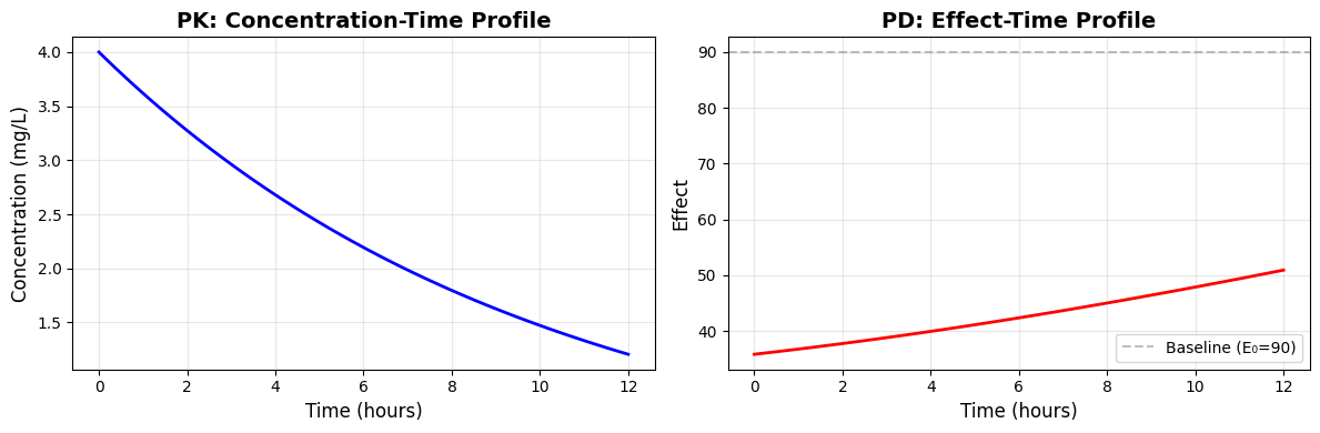
An IV bolus places the entire dose into the central compartment, so concentration decays exponentially with rate constant CL/V. We also set pharmacodynamic parameters for baseline effect, maximum effect change, and the concentration at half-maximal response.
CL, V = 5.0, 50.0            # L/h, L
E0, Emax, EC50 = 90, 65, 0.8 # effect units and concentration units

def pk_rhs(t, y):
    C = y[0]
    return [-(CL / V) * C]
Define the inhibitory Emax model and dose
The inhibitory Emax function captures how the effect falls from baseline as concentration rises. For this example we simulate a 200 mg IV bolus.
def inhibitory_emax(C):
    return E0 - (Emax * C) / (EC50 + C)

dose = 200.0                 # mg IV bolus
Solve the PK equation and compute the effect-time profile
We initialize concentration with C0 = dose/V, integrate the ODE over 12 hours, sample 100 evenly spaced time points, and map concentrations to effects through the inhibitory model.
C0 = dose / V
sol = solve_ivp(pk_rhs, [0, 12], [C0], dense_output=True)
t_grid = np.linspace(0, 12, 100)
C = sol.sol(t_grid)[0]
effect = inhibitory_emax(C)
Visualize the results
The notebook finishes by plotting both the concentration-time profile and the resulting effect-time curve, showing how the effect rebounds toward baseline as concentration declines.
Swap in your own fitted parameters and concentration predictions to explore patient-specific titration schemes or concentration thresholds.
Diagnostics tailored to direct-response models
- Plot effect vs. concentration with both observations and model-predicted curves; lack of collapse onto a single curve is the clearest sign that a direct model is insufficient.
- Examine conditional weighted residuals against concentration—systematic bias at high concentrations usually flags the need for an $E_{\max}$ or sigmoid curve.
- Run prediction-corrected VPCs focused on peak and trough time windows; misspecification often appears first at the peaks.
- Quantify parameter uncertainty (covariance matrix, bootstrap, Bayesian posterior). Direct-response dose recommendations are sensitive to $EC_{50}$ or $IC_{50}$ confidence intervals.
Communicating model results
- Translate parameters into bedside rules (e.g., “Keep concentration between 25 and 60 ng/mL to sustain >80% platelet inhibition”).
- Pair tabulated metrics with replicate clinical plots—decision-makers trust curves showing data overlays.
- Document assay conditions and any covariate effects so implementation teams can reproduce exposure-response projections.
References
- Bergström M, et al. Clin Pharmacol Ther. 2004;75:174–184.
- FDA Center for Drug Evaluation and Research. Clinical Pharmacology Review for Kengreal (cangrelor) BLA 204958; 2014.
- Vozeh S, et al. Clin Pharmacol Ther. 1983;33:22–30.