PyMC calls the introductory GLM tutorial the “Inference Button” notebook for a reason: the official guide walks through rephrasing ordinary least squares as a probabilistic program and then leans on MCMC to do the heavy lifting. This PyMC 401 recap follows that same arc with the companion notebook at content/posts/mcmc/pymc/pymc_401.ipynb. We generate synthetic data, hand-code the PyMC model, rerun it through Bambi’s Patsy-style interface, and finish with ArviZ diagnostics so you can see exactly what happens after you “press the button.”
1. From deterministic slopes to Bayesian posteriors
The tutorial starts by reminding us that classic linear regression is $Y = X\beta + \epsilon$ with a Gaussian noise term. Bayesians rewrite this as $Y \sim \mathcal{N}(X\beta, \sigma^2)$ so they can put priors on every unknown and recover full posterior distributions instead of point estimates. Those two benefits—encoding prior beliefs (e.g., “the noise scale should stay small”) and quantifying parameter uncertainty—are what make the Bayesian treatment practical even for a textbook straight line.
2. Reproducible synthetic data
Both the doc and the notebook lock in RANDOM_SEED = 8927 and fabricate a dataset with a true intercept of 1, a slope of 2, and Gaussian scatter (standard deviation 0.5). Running the cell below yields a 200-row DataFrame plus a reference line we can plot for visual checks:
size = 200
true_intercept = 1
true_slope = 2

x = np.linspace(0, 1, size)
true_regression_line = true_intercept + true_slope * x
y = true_regression_line + rng.normal(scale=0.5, size=size)

data = pd.DataFrame({"x": x, "y": y})
The tutorial explicitly encourages plotting the scatter and ground-truth line (ax.plot(x, y, "x") and ax.plot(x, true_regression_line)), because that “human eyeball test” catches oddities before you sample.
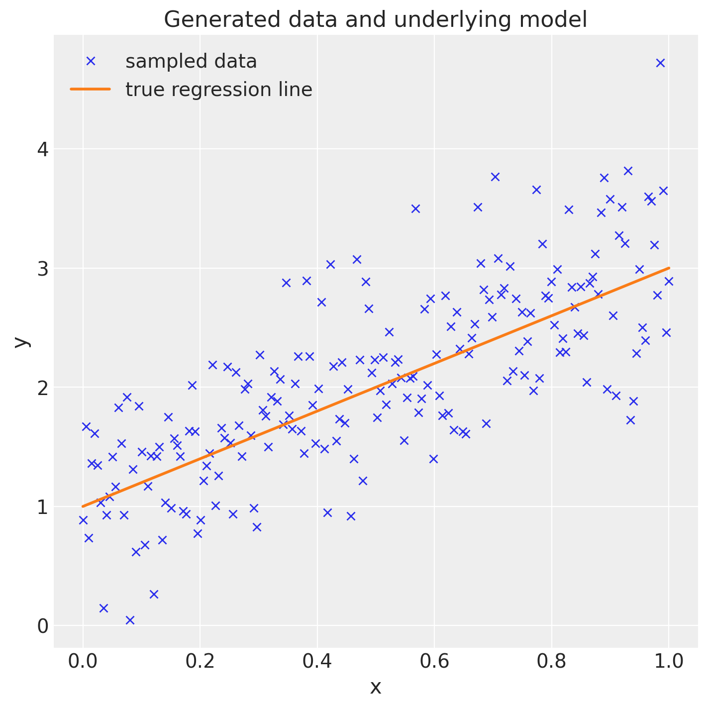
Figure 1. Synthetic GLM dataset from the PyMC 401 notebook: crosses show noisy draws, the curve is the known linear trend with slope 2.
3. Building the PyMC model by hand
Inside a pm.Model() context we place weakly informative priors—HalfCauchy for the observation noise and centered Normals for both regression terms—and express the likelihood as another Normal whose mean is intercept + slope * x. The notebook sticks with PyMC’s defaults for NUTS and simply asks for 3000 posterior draws:
with Model() as model:
    sigma = HalfCauchy("sigma", beta=10)
    intercept = Normal("Intercept", 0, sigma=20)
    slope = Normal("slope", 0, sigma=20)

    Normal("y", mu=intercept + slope * x, sigma=sigma, observed=y)

    idata = sample(3000, random_seed=RANDOM_SEED)
That short block mirrors the tutorial’s “Bayesian GLMs in PyMC” section verbatim. The heavy work is hidden inside sample, which adapts NUTS, builds the joint log-density, and returns an InferenceData bundle ready for diagnostics.
4. Replaying the fit through Bambi
PyMC’s Bambi wrapper recreates the same model with a one-line formula string ("y ~ x"). The notebook tries to import bambi as bmb and silently installs it if missing, then calls model.fit(draws=3000) to produce another InferenceData. This follows the tutorial’s advice for scientists coming from R-style model syntax: let Bambi translate Patsy formulas into PyMC components while still exposing the Model object if you need to inspect priors or add custom terms. Comparing the hand-written PyMC results with the Bambi version is a fast sanity check that the abstractions stay honest.
model = bmb.Model("y ~ x", data)
idata = model.fit(draws=3000, random_seed=RANDOM_SEED)
5. Inspecting traces and predictive lines
Once the samples land in idata, we lean on ArviZ exactly as the tutorial demonstrates:
az.plot_trace(idata, figsize=(10, 7))shows well-mixed, symmetric posteriors forIntercept,x, andsigma, confirming the priors were weak relative to the data.- To visualize fitted regressions, the notebook computes a deterministic
y_model = Intercept + x * slopeinside the posterior group and then callsaz.plot_lmwith 100 random posterior draws. The resulting family of lines should cover the original scatter while clustering tightly around the true slope.
idata.posterior["y_model"] = idata.posterior["Intercept"] + idata.posterior["x"] * xr.DataArray(x)
_, ax = plt.subplots(figsize=(7, 7))
az.plot_lm(idata=idata, y="y", num_samples=100, axes=ax, y_model="y_model")
ax.set_title("Posterior predictive regression lines")
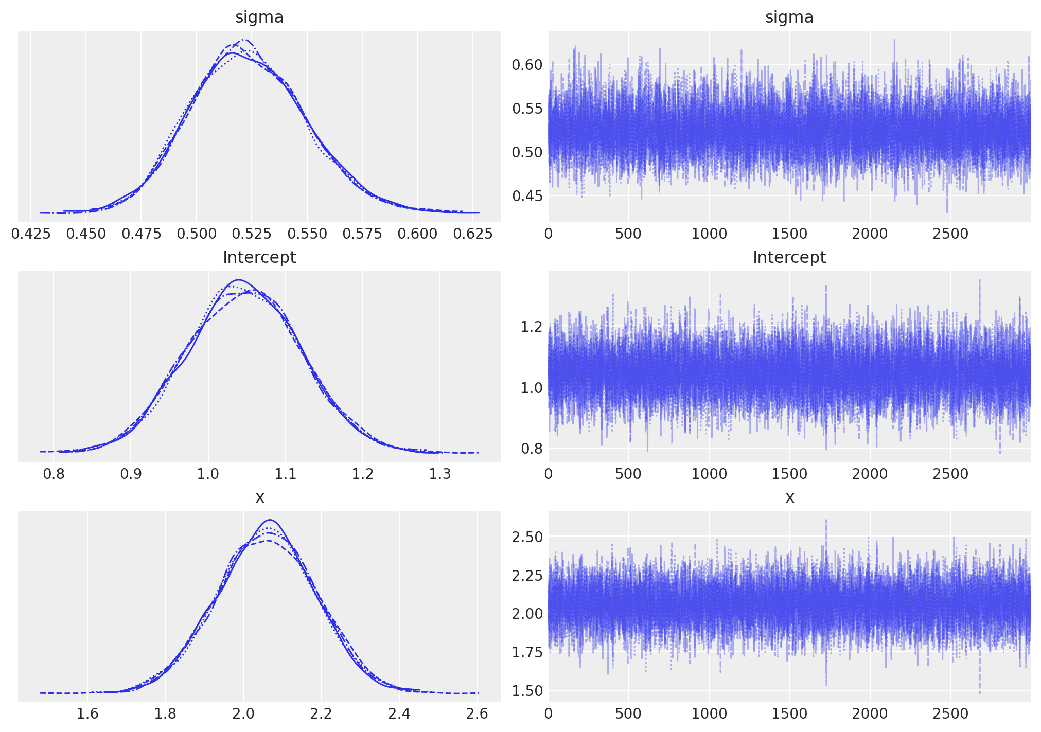
Figure 2. Posterior traces and marginal densities from the PyMC/Bambi model; chains mix well with symmetric posteriors centered near the true parameters.
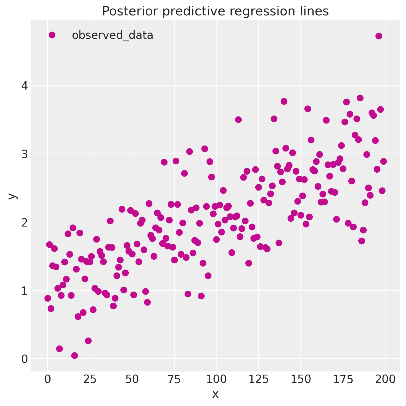
Figure 3. Posterior predictive regression fan from az.plot_lm: orange lines are random posterior fits, and the scatter points are the observed data.
These two diagnostics give you immediate feedback on whether the NUTS chains converged and whether the posterior predictive check recovers the generating process.
6. Where to experiment next
- Replay everything locally.
content/posts/mcmc/pymc/pymc_401.ipynbcontains exact cells for the imports, seeded data generation, PyMC model, Bambi fit, and ArviZ visuals so you can rerun them verbatim. - Push beyond Gaussians. The official GLM tutorial closes with ideas for extending the same workflow to logistic and Poisson GLMs—swap the likelihood, update priors, and keep the ArviZ checks.
- Tinker with priors and formula terms. Try shrinkage priors on the slope, add polynomial features (
"y ~ x + I(x ** 2)"in Bambi), or plug in new predictors to see how the trace plots and posterior predictive fan react.
Pressing the “Inference Button” gets easier when you know what each step is doing. This PyMC 401 walkthrough demystifies the pieces so you can own every part of a Bayesian straight-line regression before graduating to richer GLMs.