PyMC looks friendly on the surface, but every model you build eventually turns into a PyTensor graph. Understanding that translation is the focus of this PyMC 301 lesson, which distills the material from the upstream PyMC & PyTensor tutorial and the companion notebook at content/posts/mcmc/pymc/pymc_301.ipynb. We’ll build graphs by hand, inspect their internals, and see exactly how PyMC attaches log-probabilities and value variables under the hood.
1. From NumPy scalars to PyTensor graphs
PyTensor mirrors the NumPy API but every operation adds a node to a computation graph. Start with explicit tensor variables and wire them together:
import pytensor
import pytensor.tensor as pt
import numpy as np

x = pt.scalar("x")
y = pt.vector("y")
z = x + y
w = pt.log(z)

pytensor.dprint(w)
pytensor.dprint prints a readable graph showing each TensorVariable, its owner Op, and the chain of transformations. When you compile the graph with pytensor.function and feed numerical values, you’re executing the graph exactly as PyMC would during sampling:
f = pytensor.function(inputs=[x, y], outputs=w)
f(0, [1, np.e])  # array([0., 1.])
2. Inspecting and rewriting graphs
Every variable exposes structural metadata, so you can traverse graphs explicitly—a useful debugging trick highlighted in the PyMC tutorial:
stack = [w]
while stack:
    var = stack.pop(0)
    if var.owner is None:
        print(f"{var} is a root variable")
        continue
    print(f"{var} comes from {var.owner.op}")
    stack.extend(var.owner.inputs)
PyTensor also makes it easy to swap subgraphs. The notebook shows how to replace x + y with exp(x + y) without redefining the entire graph:
parent = w.owner.inputs[0]          # this is z
new_parent = pt.exp(parent)         # build a replacement
new_parent.name = "exp(x + y)"

new_w = pytensor.clone_replace(w, {parent: new_parent})
The resulting graph now represents $\log(\exp(x + y))$ and evaluates accordingly, demonstrating that symbolic rewrites are first-class operations.
3. Random variables bridge PyTensor and PyMC
pt.random defines distribution-aware tensors that produce new draws whenever you call .eval():
y = pt.random.normal(0, 1, name="y")
for _ in range(3):
    print(y.eval())
PyMC layers additional ergonomics on top. pm.Normal.dist returns a RandomVariable object (no model context required), and pm.draw handles vectorized sampling and seeding:
import pymc as pm

x = pm.Normal.dist(mu=0, sigma=1)
samples = pm.draw(x, draws=1_000)
This is the bridge between isolated PyTensor expressions and the stochastic building blocks that end up in a PyMC model.

Figure 1. Baseline NumPy histogram—use it as a sanity check before swapping in PyTensor random variables.
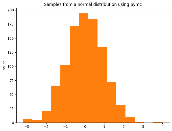
Figure 2. PyMC’s pm.draw mirrors the NumPy histogram, reinforcing that pm.Normal.dist + pm.draw gives the same samples while staying inside the PyTensor graph world.
4. Building a PyMC model atop PyTensor
Once you enter a model context, PyMC wires its RandomVariables into a shared graph:
with pm.Model() as model:
    z = pm.Normal("z", mu=np.array([0, 0]), sigma=np.array([1, 2]))

pytensor.dprint(z)
model.basic_RVs   # [z]
The blog notebook demonstrates how to pull samples (pm.draw(z)) and visualize them (plt.hist2d(...)) to confirm that this vector RV really is two correlated Normals with different scales.
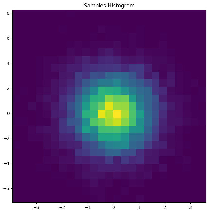
Figure 3. Joint histogram of the two-component Normal z. Even simple multivariate draws are easier to debug when you can see the geometry.
5. Seeing the log-probability graph
PyMC hooks each random variable to a log-probability node so samplers can evaluate posteriors. You can access that symbolic log-prob while still inside Python:
z_value = pt.vector("z")
z_logp = pm.logp(z, z_value)

float(z_logp.eval({z_value: [0, 0]}))
For the toy model, the result matches scipy.stats.norm.logpdf([0, 0], [0, 0], [1, 2]), confirming that PyMC and SciPy agree on the density.
If you need a callable, compile the graph:
logp_fn = model.compile_logp(sum=False)
point = model.initial_point()
logp_fn(point)
sum=False returns one entry per random variable, which is helpful for debugging multi-term models.
6. Value variables and their role
Every RandomVariable has a companion value variable that represents the unconstrained parameter PyMC actually samples. Access both mappings to understand transformations (e.g., the HalfNormal sigma is sampled on the log scale):
with pm.Model() as model_2:
    mu = pm.Normal("mu", mu=0, sigma=2)
    sigma = pm.HalfNormal("sigma", sigma=3)
    x = pm.Normal("x", mu=mu, sigma=sigma)

mu_value = model_2.rvs_to_values[mu]
sigma_value = model_2.rvs_to_values[sigma]
x_value = model_2.rvs_to_values[x]
Stacking model_2.logp(sum=False) and evaluating at a manually specified dictionary recovers the same numbers as direct SciPy calls, validating that you can trace every log-prob computation back to classic probability density functions.
7. Where to go next
- Open
content/posts/mcmc/pymc/pymc_301.ipynbto execute every code cell shown above. - Use
pytensor.dprintandmodel.compile_logpwhenever a sampler misbehaves; they expose the exact graph that drives inference. - Explore the rest of the PyMC & PyTensor tutorial for sections on Graphviz visualization, optimizer passes, and more advanced graph surgery ideas.
Once you’re comfortable manipulating PyTensor graphs directly, PyMC models stop feeling like black boxes—you can read, rewrite, and validate every symbolic piece that contributes to the posterior.