Predictive checks are essential tools in the Bayesian workflow, bridging the gap between abstract posterior distributions and real-world model validation. This post walks through the PyMC predictive checks tutorial, demonstrating how to use prior predictive checks to validate assumptions before seeing data and posterior predictive checks (PPCs) to assess whether your fitted model can reproduce observed patterns. By the end you’ll understand how to simulate from priors, diagnose model fit through visual comparisons, and generate out-of-sample predictions with uncertainty quantification.
Why predictive checks matter
- Prior predictive checks reveal whether your priors encode reasonable assumptions about the data-generating process before you look at observations
- Posterior predictive checks assess whether the fitted model can reproduce patterns in the observed data—if not, the model may be misspecified
- Out-of-sample prediction with full posterior uncertainty is straightforward once you’ve set up mutable data containers
- Visual diagnostics make model criticism accessible to collaborators and stakeholders who don’t read trace plots
The philosophy: criticism under the frequentist lens
As the Edward documentation explains:
PPCs are an excellent tool for revising models, simplifying or expanding the current model as one examines how well it fits the data. They are inspired by prior checks and classical hypothesis testing, under the philosophy that models should be criticized under the frequentist perspective of large sample assessment.
PPCs can be applied to hypothesis testing, model comparison, and model averaging, but their primary value is holistic model criticism: perform many checks to understand fit quality from multiple angles, not just a single pass/fail test.
Setup and data generation
We’ll build two examples: a linear regression with standardized predictors and a logistic regression for binary outcomes.
import arviz as az
import matplotlib.pyplot as plt
import numpy as np
import xarray as xr
from scipy.special import expit as logistic
import pymc as pm

print(f"Running on PyMC v{pm.__version__}")
# Running on PyMC v5.26.1

az.style.use("arviz-darkgrid")

RANDOM_SEED = 58
rng = np.random.default_rng(RANDOM_SEED)

def standardize(series):
    """Standardize a pandas series"""
    return (series - series.mean()) / series.std()
Example 1: Linear regression with prior checks
Simulating non-standard data
We intentionally generate data with high variance to mimic real-world scenarios:
N = 100

true_a, true_b, predictor = 0.5, 3.0, rng.normal(loc=2, scale=6, size=N)
true_mu = true_a + true_b * predictor
true_sd = 2.0

outcome = rng.normal(loc=true_mu, scale=true_sd, size=N)

f"{predictor.mean():.2f}, {predictor.std():.2f}, {outcome.mean():.2f}, {outcome.std():.2f}"
# Output: '1.59, 5.69, 4.97, 17.54'
The predictor has mean ~1.6 and standard deviation ~5.7, while the outcome has even larger spread (~17.5). This high variance can confuse samplers, motivating standardization:
predictor_scaled = standardize(predictor)
outcome_scaled = standardize(outcome)

f"{predictor_scaled.mean():.2f}, {predictor_scaled.std():.2f}, {outcome_scaled.mean():.2f}, {outcome_scaled.std():.2f}"
# Output: '0.00, 1.00, -0.00, 1.00'
After standardizing, both variables have mean 0 and standard deviation 1, creating a friendlier geometry for NUTS.
Prior predictive check with flat priors
Let’s start with conventional “flat” priors and see what they imply:
with pm.Model() as model_1:
    a = pm.Normal("a", 0.0, 10.0)
    b = pm.Normal("b", 0.0, 10.0)

    mu = a + b * predictor_scaled
    sigma = pm.Exponential("sigma", 1.0)

    pm.Normal("obs", mu=mu, sigma=sigma, observed=outcome_scaled)
    idata = pm.sample_prior_predictive(draws=50, random_seed=rng)
What do these priors mean? It’s hard to tell from the specification alone—plotting is essential:
_, ax = plt.subplots()

x = xr.DataArray(np.linspace(-2, 2, 50), dims=["plot_dim"])
prior = idata.prior
y = prior["a"] + prior["b"] * x

ax.plot(x, y.stack(sample=("chain", "draw")), c="k", alpha=0.4)
ax.set_xlabel("Predictor (stdz)")
ax.set_ylabel("Mean Outcome (stdz)")
ax.set_title("Prior predictive checks -- Flat priors");
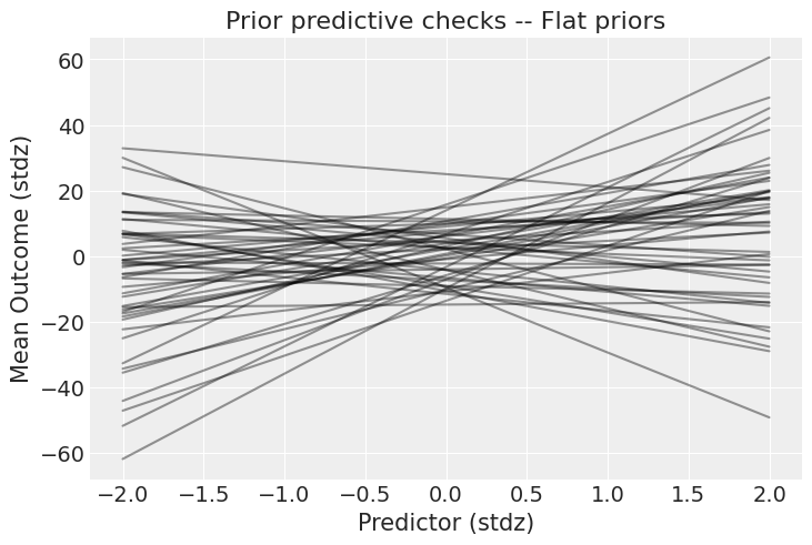
Figure 1. Prior predictive check with flat priors. The y-axis spans from -40 to +40 standard deviations—these priors allow absurdly strong relationships that are implausible in most real-world settings.
The plot reveals that flat priors $\mathcal{N}(0, 10)$ on the intercept and slope allow the outcome to range from −40 to +40 standard deviations. This is far too permissive—we’re essentially saying we have no information about the relationship, which is rarely true. Time to tighten the screws.
Prior predictive check with weakly regularizing priors
Following weakly informative prior recommendations, we shrink the prior standard deviations:
with pm.Model() as model_1:
    a = pm.Normal("a", 0.0, 0.5)
    b = pm.Normal("b", 0.0, 1.0)

    mu = a + b * predictor_scaled
    sigma = pm.Exponential("sigma", 1.0)

    pm.Normal("obs", mu=mu, sigma=sigma, observed=outcome_scaled)
    idata = pm.sample_prior_predictive(draws=50, random_seed=rng)
Plotting again:
_, ax = plt.subplots()

x = xr.DataArray(np.linspace(-2, 2, 50), dims=["plot_dim"])
prior = idata.prior
y = prior["a"] + prior["b"] * x

ax.plot(x, y.stack(sample=("chain", "draw")), c="k", alpha=0.4)
ax.set_xlabel("Predictor (stdz)")
ax.set_ylabel("Mean Outcome (stdz)")
ax.set_title("Prior predictive checks -- Weakly regularizing priors");
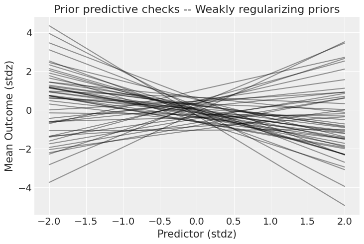
Figure 2. Prior predictive check with weakly regularizing priors. The outcome now stays within ±4 standard deviations, a much more plausible range. The priors still allow both weak and strong relationships, but exclude pathological extremes.
Much better! The outcome stays within ±4 standard deviations, a realistic range for standardized data. These priors still permit a wide variety of relationships (weak or strong, positive or negative) but rule out the absurd extremes that flat priors allowed.
Key lesson: Prior predictive checks turn abstract prior specifications into concrete implications on the outcome scale. Always visualize before fitting.
Sampling the posterior
With validated priors, we sample:
with model_1:
    idata.extend(pm.sample(1000, tune=2000, random_seed=rng))

az.plot_trace(idata);
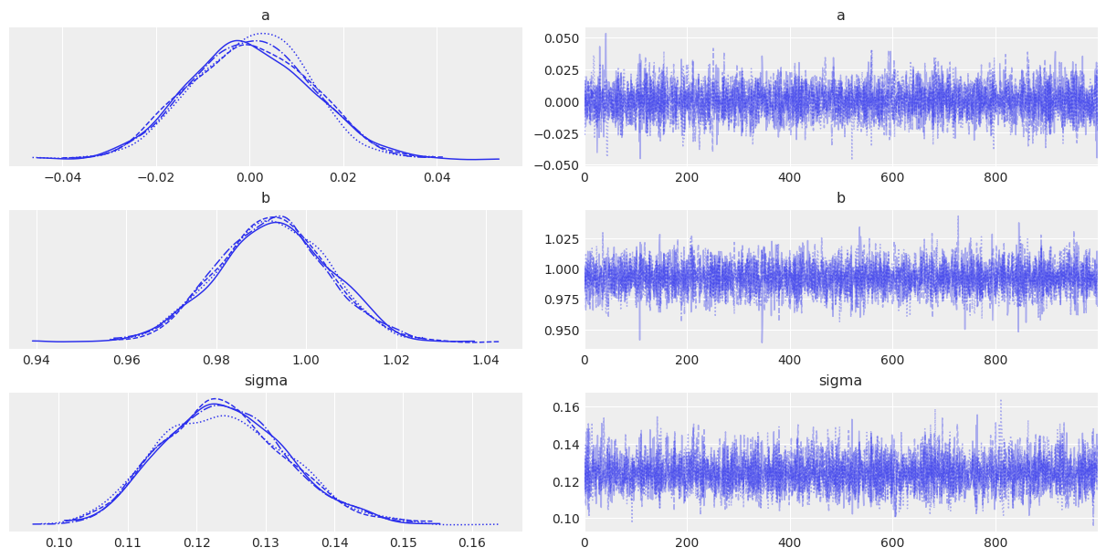
Figure 3. Trace plot for the linear regression. Left: posterior distributions for intercept a, slope b, and residual standard deviation sigma. Right: MCMC traces showing good mixing with no trends or divergences. All chains converged successfully.
The trace plots confirm convergence: chains are well-mixed, marginal distributions are smooth, and there are no divergences. The posterior is ready for interpretation.
Posterior predictive checks
Now we generate synthetic datasets from the posterior and compare them to observed data:
with model_1:
    pm.sample_posterior_predictive(idata, extend_inferencedata=True, random_seed=rng)
This draws 4000 posterior samples (4 chains × 1000 draws), and for each sample, generates $N=100$ synthetic observations using that sample’s $a$, $b$, and $\sigma$ values. The result is 4000 simulated datasets stored in idata.posterior_predictive.
ArviZ’s plot_ppc overlays these simulated datasets with the observed data:
az.plot_ppc(idata, num_pp_samples=100);
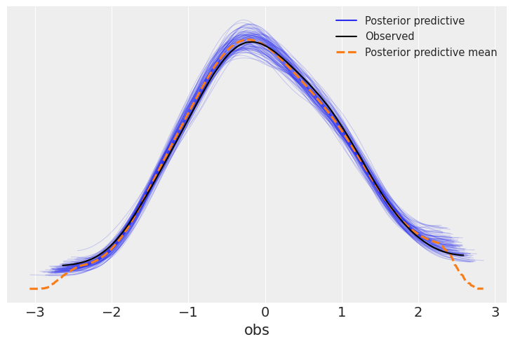
Figure 4. Posterior predictive check. The blue curves are kernel density estimates from 100 simulated datasets drawn from the posterior. The black curve is the observed data. The model successfully reproduces the shape and spread of the observed distribution, indicating good fit.
Interpretation: The observed data (black) falls well within the range of simulated datasets (blue). The model captures the central tendency and spread of the data. If the observed curve were far outside the simulated range, we’d suspect model misspecification.
Custom predictive plot with uncertainty
Generic PPCs are useful, but domain-specific visualizations are often more informative. Let’s plot the posterior mean function with highest density intervals (HDIs):
post = idata.posterior
mu_pp = post["a"] + post["b"] * xr.DataArray(predictor_scaled, dims=["obs_id"])

_, ax = plt.subplots()

ax.plot(
    predictor_scaled,
    mu_pp.mean(("chain", "draw")),
    label="Mean outcome",
    color="C1",
    alpha=0.6
)
ax.scatter(predictor_scaled, idata.observed_data["obs"])
az.plot_hdi(predictor_scaled, idata.posterior_predictive["obs"])

ax.set_xlabel("Predictor (stdz)")
ax.set_ylabel("Outcome (stdz)");
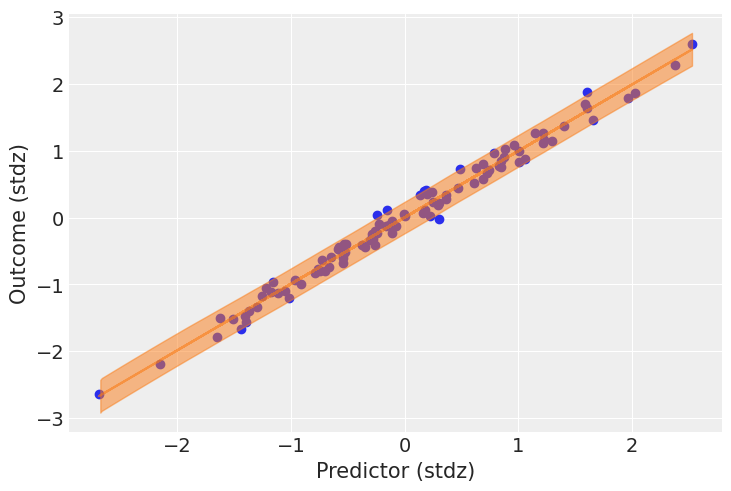
Figure 5. Posterior fit visualization. Orange line: posterior mean of the linear relationship. Blue shaded region: 94% HDI for individual predictions (includes both parameter and residual uncertainty). Black points: observed data. The narrow orange band reflects low uncertainty in the mean function; the wide blue HDI captures individual-level variability.
What this shows:
- Orange line: Posterior mean of $\mu = a + b \cdot \text{predictor}$—the expected outcome for each predictor value
- Blue shaded region: 94% HDI for individual predictions from
posterior_predictive["obs"], incorporating both parameter uncertainty and residual noise $\sigma$ - Black points: Observed data
The tight orange band around the mean indicates low uncertainty in the estimated relationship (we have 100 observations). The wide blue HDI reflects the intrinsic variability captured by $\sigma$—even with perfect knowledge of $a$, $b$, and $\sigma$, individual outcomes scatter around the mean.
Example 2: Logistic regression with out-of-sample prediction
Binary outcome data generation
Now we move to classification with a logistic regression:
N = 400
true_intercept = 0.2
true_slope = 1.0
predictors = rng.normal(size=N)
true_p = logistic(true_intercept + true_slope * predictors)

outcomes = rng.binomial(1, true_p)
outcomes[:10]
# Output: array([1, 1, 1, 0, 1, 0, 0, 1, 1, 0])
The predictor is standard normal, transformed through the logistic function to produce success probabilities, then converted to binary outcomes via Bernoulli sampling.
Model specification with mutable data
To enable out-of-sample prediction, we wrap the predictor in pm.Data:
with pm.Model() as model_2:
    betas = pm.Normal("betas", mu=0.0, sigma=np.array([0.5, 1.0]), shape=2)

    # Set predictors as mutable data for easy updates:
    pred = pm.Data("pred", predictors, dims="obs_id")
    p = pm.Deterministic("p", pm.math.invlogit(betas[0] + betas[1] * pred), dims="obs_id")

    outcome = pm.Bernoulli("outcome", p=p, observed=outcomes, dims="obs_id")

    idata_2 = pm.sample(1000, tune=2000, return_inferencedata=True, random_seed=rng)

az.summary(idata_2, var_names=["betas"], round_to=2)
| Parameter | mean | sd | hdi_3% | hdi_97% | ess_bulk | r_hat |
|---|---|---|---|---|---|---|
| betas[0] | 0.22 | 0.11 | 0.03 | 0.43 | 4002.84 | 1.0 |
| betas[1] | 1.02 | 0.14 | 0.77 | 1.29 | 4079.89 | 1.0 |
Key findings:
- The intercept estimate (0.22) is close to the true value (0.20)
- The slope estimate (1.02) nearly matches the true slope (1.00)
- High effective sample sizes (ESS > 4000) and $\hat{R} = 1.0$ confirm excellent convergence
Why pm.Data? By declaring pred as mutable data, we can later swap in new predictor values without rebuilding the model graph—essential for prediction workflows.
Out-of-sample prediction
Generate new test data and update the model:
predictors_out_of_sample = rng.normal(size=50)
outcomes_out_of_sample = rng.binomial(
    1, logistic(true_intercept + true_slope * predictors_out_of_sample)
)

with model_2:
    # Update predictor values:
    pm.set_data({"pred": predictors_out_of_sample})

    # Sample posterior predictive with the new predictors:
    idata_2 = pm.sample_posterior_predictive(
        idata_2,
        var_names=["p"],
        return_inferencedata=True,
        predictions=True,
        extend_inferencedata=True,
        random_seed=rng,
    )
What happened:
pm.set_datareplaced the training predictors with out-of-sample valuespm.sample_posterior_predictiveused the posterior draws ofbetasto compute predicted probabilitiespfor the new predictorspredictions=Truestores results inidata_2.predictionsinstead of overwritingposterior_predictive
Visualizing predictions with uncertainty
_, ax = plt.subplots(figsize=(12, 6))

preds_out_of_sample = idata_2.predictions_constant_data.sortby("pred")["pred"]
model_preds = idata_2.predictions.sortby(preds_out_of_sample)

# Uncertainty about the estimates (HDI):
ax.vlines(
    preds_out_of_sample,
    *az.hdi(model_preds)["p"].transpose("hdi", ...),
    alpha=0.8,
)

# Expected probability of success:
ax.plot(
    preds_out_of_sample,
    model_preds["p"].mean(("chain", "draw")),
    "o",
    ms=5,
    color="C1",
    alpha=0.8,
    label="Expected prob.",
)

# Actual outcomes:
ax.scatter(
    x=predictors_out_of_sample,
    y=outcomes_out_of_sample,
    marker="x",
    color="k",
    alpha=0.8,
    label="Observed outcomes",
)

# True probabilities:
x = np.linspace(predictors_out_of_sample.min() - 0.1, predictors_out_of_sample.max() + 0.1)
ax.plot(
    x,
    logistic(true_intercept + true_slope * x),
    lw=2,
    ls="--",
    color="#565C6C",
    alpha=0.8,
    label="True prob.",
)

ax.set_xlabel("Predictor")
ax.set_ylabel("Prob. of success")
ax.set_title("Out-of-sample Predictions")
ax.legend(fontsize=10, frameon=True, framealpha=0.5);
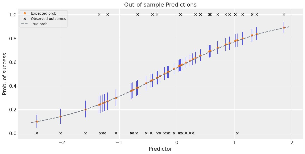
Figure 6. Out-of-sample predictions for logistic regression. Orange dots: posterior mean probability of success for each test case. Vertical blue lines: 94% HDI capturing parameter uncertainty. Black X’s: actual binary outcomes. Dashed grey line: true probability function (oracle, unknown in practice). The model’s predictions closely track the true probabilities, and most observed outcomes fall within the predicted uncertainty bands.
Reading the plot:
- Orange dots: Posterior mean of $p = \text{logit}^{-1}(\beta_0 + \beta_1 \cdot \text{pred})$ for each test predictor
- Vertical blue lines: 94% HDI for each prediction, quantifying parameter uncertainty
- Black X’s: Actual binary outcomes (0 or 1)—they don’t always align with high-probability predictions because the process is stochastic
- Dashed grey curve: True probability function (only known because we simulated the data)
The model’s predicted probabilities closely follow the true curve, demonstrating excellent out-of-sample calibration. Some observed outcomes (0’s when $p$ is high, or 1’s when $p$ is low) are mismatches, but this is expected: even a perfectly calibrated model can’t predict individual coin flips, only their probabilities.
Best practices for predictive checks
Prior predictive checks
- ✅ Always visualize prior implications on the outcome scale before fitting
- ✅ Check extremes: ensure priors don’t permit absurd scenarios (e.g., outcomes spanning hundreds of standard deviations)
- ✅ Incorporate domain knowledge: use weakly informative priors that encode reasonable constraints
- ✅ Test sampler behavior: tight priors can prevent initialization failures in complex models
Posterior predictive checks
- ✅ Use multiple visualizations: generic density overlays (ArviZ’s
plot_ppc) plus domain-specific plots - ✅ Look for systematic deviations: if observed data consistently falls outside simulated ranges, revise the model
- ✅ Check summary statistics: compare means, variances, skewness, or quantiles between observed and simulated datasets
- ✅ Don’t over-interpret single checks: perform many PPCs to get a holistic sense of fit
Out-of-sample prediction
- ✅ Use
pm.Datafor predictors you’ll want to update later - ✅ Set
predictions=Trueto avoid overwriting in-sample PPCs - ✅ Visualize uncertainty: show HDIs or credible intervals, not just point predictions
- ✅ Validate on held-out data when possible, not just simulated test sets
Predictive checks vs. other diagnostics
How PPCs differ from trace plots and convergence diagnostics:
- Trace plots assess sampler behavior—did NUTS explore the posterior efficiently?
- Convergence metrics ($\hat{R}$, ESS) check numerical reliability—can we trust the posterior samples?
- Predictive checks evaluate model adequacy—does the fitted model match reality?
All three are necessary. A well-converged sampler can still produce a terrible model if the likelihood or priors are misspecified.
When to prefer LOO/WAIC over PPCs:
- Model comparison: LOO and WAIC provide quantitative rankings across multiple models (see PyMC 202)
- Out-of-sample performance: LOO estimates predictive accuracy without re-running the sampler
- Pareto diagnostics: LOO flags influential observations that PPCs might miss
When PPCs are superior:
- Interpretability: stakeholders can grasp “does the model produce realistic data?” more easily than “what is the elpd_loo?”
- Exploratory analysis: PPCs are open-ended—you can check any aspect of the data (means, tails, correlations) without predefining a loss function
- Model revision: visualizing mismatches guides concrete model improvements (add interactions, change link functions, etc.)
Use both approaches in practice: PPCs for intuition and exploration, LOO/WAIC for formal comparisons.
Workflow integration
A complete Bayesian workflow incorporates predictive checks at multiple stages:
- Pre-data: Prior predictive checks validate assumptions and help communicate model structure to domain experts
- Post-fitting: Posterior predictive checks assess whether the model reproduces observed patterns
- Decision-making: Out-of-sample predictions with uncertainty inform real-world actions (treatment assignment, resource allocation, etc.)
- Iteration: When PPCs reveal poor fit, revise the model (richer likelihood, better priors, additional predictors) and repeat
This cycle mirrors the scientific method: hypothesize (specify priors), test (fit and check), revise (update model), and iterate.
Summary
We demonstrated two core tools in the Bayesian modeling toolkit:
Prior predictive checks revealed that “flat” priors $\mathcal{N}(0, 10)$ allow absurd relationships (outcomes spanning ±40 SD), while weakly regularizing priors $\mathcal{N}(0, 1)$ stay within plausible ranges (±4 SD). Always visualize prior implications before fitting.
Posterior predictive checks confirmed that the fitted linear regression reproduced the observed data’s distribution. Custom plots with HDIs quantified uncertainty in both the mean function and individual predictions.
Out-of-sample prediction for logistic regression demonstrated how
pm.Dataenables seamless predictor updates without rebuilding the model. Predicted probabilities closely tracked true values, with realistic uncertainty bands.
Predictive checks complement trace plots and information criteria, providing intuitive visual diagnostics for model criticism and communication. Integrate them at every stage: prior checks to validate assumptions, posterior checks to assess fit, and predictive intervals to quantify uncertainty in new settings.
References
- PyMC Posterior Predictive Checks Tutorial
- Gelman, A., Carlin, J. B., Stern, H. S., & Rubin, D. B. (2013). Bayesian Data Analysis (3rd ed.). CRC Press. (Chapter 6: Model Checking)
- Gabry, J., Simpson, D., Vehtari, A., Betancourt, M., & Gelman, A. (2019). Visualization in Bayesian workflow. Journal of the Royal Statistical Society: Series A, 182(2), 389–402.
- Stan Prior Choice Recommendations
Next steps
- PyMC 101 covers the basics of model building and sampling
- PyMC 102 introduces posterior predictive checks in a regularized regression context
- PyMC 202 discusses model comparison with LOO and WAIC
- PyMC 104 explores advanced diagnostics and convergence checks
Explore the full notebook with executable code and additional visualizations.