Model comparison is central to Bayesian workflow: you fit competing models to the same data, then rank them by out-of-sample predictive accuracy. This post walks through the PyMC model comparison tutorial, implementing the classic 8 schools example with two candidate structures—a pooled model and a hierarchical model—and comparing them using LOO cross-validation and WAIC. By the end you will understand how to compute information criteria with ArviZ, interpret Pareto k diagnostics, and decide when model differences are meaningful given uncertainty.
Why model comparison matters
- Out-of-sample prediction is the gold standard for model quality; in-sample fit alone rewards overfitting.
- Information criteria (LOO, WAIC) estimate predictive accuracy without rerunning your sampler on held-out folds.
- Pareto smoothing stabilizes importance-weighted estimates, turning naïve leave-one-out into a single-pass diagnostic.
- Standard errors on the difference between models tell you whether a gap in LOO/WAIC is real or noise.
The 8 schools dataset
We analyze treatment effects from a coaching intervention across eight schools. Each school reports an observed effect $y_j$ with known standard error $\sigma_j$; the question is whether a single pooled effect or a hierarchical (partially pooled) structure better predicts new schools.
import arviz as az
import numpy as np
import pymc as pm

print(f"Running on PyMC v{pm.__version__}")
# Running on PyMC v5.26.1

az.style.use("arviz-darkgrid")

y = np.array([28, 8, -3, 7, -1, 1, 18, 12])
sigma = np.array([15, 10, 16, 11, 9, 11, 10, 18])
J = len(y)
The data include large uncertainties ($\sigma_j$ ranges from 9 to 18), so estimating school-specific effects is challenging.
Model 1: Pooled (complete pooling)
The simplest approach assumes all schools share a single latent effect $\mu$:
$$ \mu \sim \text{Normal}(0, 10^6),\quad y_j \sim \text{Normal}(\mu, \sigma_j). $$In code:
with pm.Model() as pooled:
    mu = pm.Normal("mu", 0, sigma=1e6)
    obs = pm.Normal("obs", mu, sigma=sigma, observed=y)
    trace_p = pm.sample(2000)
The trace plot confirms good mixing for the scalar parameter $\mu$. Because there is no between-school variation, the pooled model is fast to sample and has minimal complexity.
az.plot_trace(trace_p);
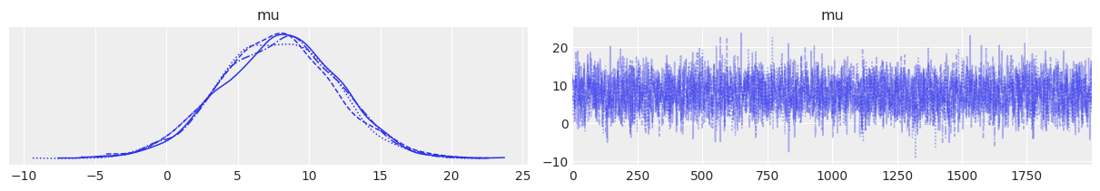
Figure 1. Trace plot for the pooled model. Left: posterior distribution of μ. Right: MCMC trace showing good mixing across 2000 samples.
Model 2: Hierarchical (partial pooling)
A hierarchical model introduces school-specific effects $\theta_j$ drawn from a common distribution:
$$ \begin{align} \mu &\sim \text{Normal}(0, 10),\quad \tau \sim \text{HalfNormal}(10),\\ \eta_j &\sim \text{Normal}(0, 1),\quad \theta_j = \mu + \tau \eta_j,\\ y_j &\sim \text{Normal}(\theta_j, \sigma_j). \end{align} $$The non-centered parameterization ($\theta_j = \mu + \tau \eta_j$) reduces posterior correlation and improves sampler efficiency when $\tau$ is small. Implementation:
with pm.Model() as hierarchical:
    eta = pm.Normal("eta", 0, 1, shape=J)
    mu = pm.Normal("mu", 0, sigma=10)
    tau = pm.HalfNormal("tau", 10)
    theta = pm.Deterministic("theta", mu + tau * eta)
    obs = pm.Normal("obs", theta, sigma=sigma, observed=y)
    trace_h = pm.sample(2000, target_accept=0.9)
We can visualize the posterior for the population mean $\mu$:
az.plot_trace(trace_h, var_names="mu");
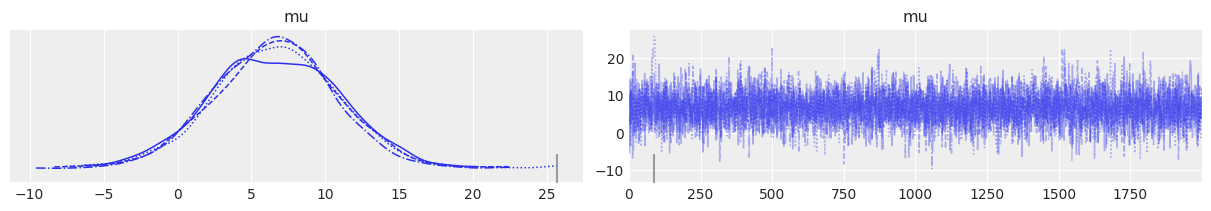
Figure 2. Trace plot for the hierarchical model’s population mean μ. The posterior is similar to the pooled model but slightly wider due to the hierarchical structure.
A forest plot of $\theta_j$ reveals shrinkage toward the population mean $\mu$; schools with high measurement error are pulled more strongly toward the center:
az.plot_forest(trace_h, var_names="theta");
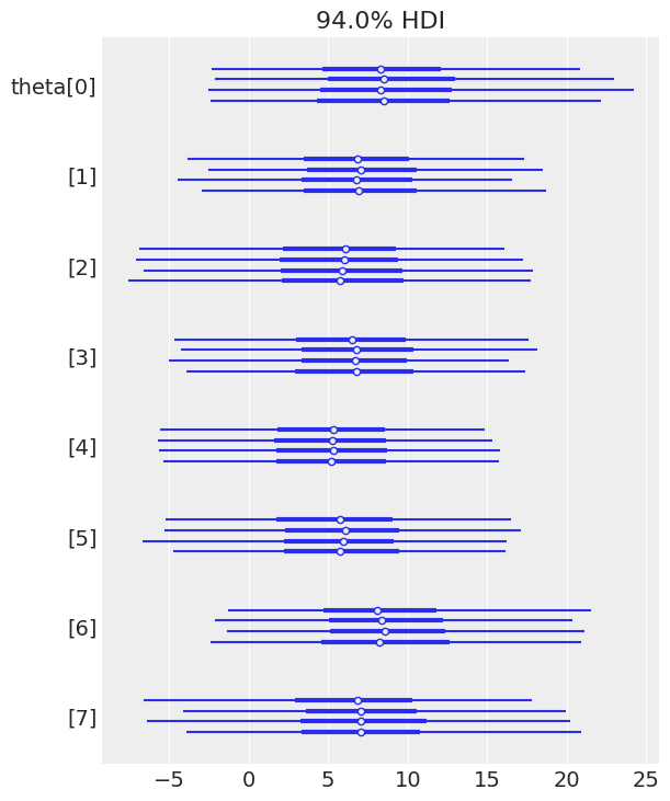
Figure 3. Forest plot of school-specific effects θⱼ. Each school has its own effect estimate, but partial pooling shrinks extreme values toward the population mean. Schools with larger measurement errors (wider intervals) are shrunk more aggressively.
Computing information criteria
To compare models, we need element-wise log-likelihoods. PyMC’s compute_log_likelihood attaches these to the trace:
with pooled:
    pm.compute_log_likelihood(trace_p)

pooled_loo = az.loo(trace_p)
print(pooled_loo)
Output:
Computed from 8000 posterior samples and 8 observations log-likelihood matrix.

         Estimate       SE
elpd_loo   -30.57     1.10
p_loo        0.68        -
------

Pareto k diagnostic values:
                         Count   Pct.
(-Inf, 0.70]   (good)        8  100.0%
   (0.70, 1]   (bad)         0    0.0%
   (1, Inf)   (very bad)    0    0.0%
Key metrics:
elpd_loo: Expected log pointwise predictive density (higher is better).p_loo: Effective number of parameters; ~0.68 is close to 1, confirming the single-parameter structure.- Pareto k < 0.7 for all observations indicates the LOO estimate is reliable.
Repeat for the hierarchical model:
with hierarchical:
    pm.compute_log_likelihood(trace_h)

hierarchical_loo = az.loo(trace_h)
print(hierarchical_loo)
Output:
Computed from 8000 posterior samples and 8 observations log-likelihood matrix.

         Estimate       SE
elpd_loo   -30.84     1.06
p_loo        1.18        -
------

Pareto k diagnostic values:
                         Count   Pct.
(-Inf, 0.70]   (good)        8  100.0%
   (0.70, 1]   (bad)         0    0.0%
   (1, Inf)   (very bad)    0    0.0%
The hierarchical model has higher effective parameter count (p_loo = 1.18) and slightly worse elpd_loo (−30.84 vs. −30.57), but the difference is small relative to standard errors.
Direct comparison with az.compare
ArviZ’s compare function computes LOO for multiple models and reports the difference:
df_comp_loo = az.compare({"hierarchical": trace_h, "pooled": trace_p})
df_comp_loo
| Model | rank | elpd_loo | p_loo | elpd_diff | weight | se | dse | warning | scale |
|---|---|---|---|---|---|---|---|---|---|
| pooled | 0 | −30.57 | 0.68 | 0.00 | 1.0 | 1.10 | 0.00 | False | log |
| hierarchical | 1 | −30.84 | 1.18 | 0.27 | 0.0 | 1.06 | 0.23 | False | log |
Column guide:
rank: 0 = best model.elpd_loo: Expected log predictive density (higher is better on the log scale).p_loo: Effective parameter count; penalizes model complexity.elpd_diff: Difference from the top model (always 0 for rank 0).weight: Stacking weights; loosely the probability each model is “best” given the data. Here the pooled model gets weight 1.0.se: Standard error ofelpd_loo.dse: Standard error of the difference. Accounts for correlation between model uncertainties. The difference (0.27) is small relative todse(0.23), so the models are essentially tied.warning: Flags unreliable LOO estimates (none here).scale: Reporting scale; default is log (higher is better). Other options: deviance (lower is better), negative-log (lower is better).
Visual comparison
az.plot_compare(df_comp_loo, insample_dev=False);

Figure 4. Model comparison visualization. The pooled model (top) has a slightly higher elpd_loo (better predictive accuracy), shown by the vertical dashed reference line. The hierarchical model’s circle is shifted left, with the triangle indicating the difference. The grey error bar on the triangle (standard error of the difference) shows substantial uncertainty, indicating the models are essentially equivalent.
The plot (inspired by Richard McElreath’s Statistical Rethinking) shows:
- Empty circles:
elpd_loofor each model. - Black error bars: Standard error of
elpd_loo. - Vertical dashed line: Best model’s
elpd_loo. - Triangles: Difference from the best model.
- Grey error bars on triangles: Standard error of the difference (
dse).
In this case the triangle for the hierarchical model nearly overlaps zero once you account for dse, confirming no strong preference.
Interpretation: why are the models so close?
Though the hierarchical model is more realistic (schools differ), it offers little predictive advantage here:
- Small sample size: Eight schools is barely enough to estimate a population variance $\tau$.
- High measurement error: The $\sigma_j$ are large, obscuring true between-school variation.
- Shrinkage toward pooling: When data are noisy, partial pooling pulls school effects toward the grand mean, converging on the pooled model’s behavior.
Practical implications
- Standard errors matter. The 0.27 difference is smaller than the 0.23
dse, so the gap is not statistically meaningful. - Choose on theory. If you expect heterogeneity across schools (or plan to generalize to new schools), the hierarchical model is still justified even if LOO doesn’t strongly favor it.
- Compute both LOO and WAIC. They usually agree, but checking both guards against pathological cases.
LOO vs. WAIC
LOO (Pareto-smoothed importance sampling):
- Approximates exact leave-one-out cross-validation.
- Provides Pareto k diagnostics to detect unreliable estimates.
- Generally preferred; ArviZ uses it by default.
WAIC (Watanabe–Akaike information criterion):
- Fully Bayesian; computes log pointwise predictive density + effective parameter penalty.
- Faster than re-running LOO from scratch (though PSIS-LOO is also one-pass).
- No Pareto diagnostics, so less robust in edge cases.
Both are valid. Use LOO when you want diagnostic feedback; use WAIC for quick historical comparisons or when your workflow is already tuned to it.
Best practices checklist
- ✅ Check Pareto k < 0.7 for all observations; if k > 0.7, LOO may be unstable (consider K-fold CV).
- ✅ Report both point estimates and standard errors (
se,dse); differences smaller thandseare inconclusive. - ✅ Visualize with
az.plot_compareto see uncertainty overlap at a glance. - ✅ Combine information criteria with posterior predictive checks and domain knowledge; LOO alone doesn’t guarantee the model is useful.
- ✅ Use non-centered parameterizations in hierarchical models to improve sampler efficiency and stabilize LOO estimates.
Summary
We compared a pooled and hierarchical model for the 8 schools dataset using LOO cross-validation:
- The pooled model (
elpd_loo = −30.57) slightly outperformed the hierarchical model (elpd_loo = −30.84), but the 0.27 difference is smaller than the standard error of the difference (0.23). - Both models have reliable Pareto k diagnostics (all k < 0.7).
- The hierarchical model’s higher effective parameter count (
p_loo = 1.18vs. 0.68) didn’t translate to better predictive accuracy, likely because the data are too sparse to precisely estimate between-school variation. - In practice you might still prefer the hierarchical model for theoretical reasons (schools do differ) and for generalizing to new schools, even when LOO doesn’t declare a clear winner.
Model comparison is a tool, not a verdict. Use it alongside subject-matter expertise, posterior predictive checks, and sensitivity analyses to build defensible Bayesian workflows.
References
- Gelman, A., Hwang, J., & Vehtari, A. (2014). Understanding predictive information criteria for Bayesian models. Statistics and Computing, 24(6), 997–1016.
- Vehtari, A., Gelman, A., & Gabry, J. (2016). Practical Bayesian model evaluation using leave-one-out cross-validation and WAIC. Statistics and Computing, 27(5), 1413–1432.
- Watanabe, S. (2010). Asymptotic equivalence of Bayes cross validation and widely applicable information criterion in singular learning theory. Journal of Machine Learning Research, 11, 3571–3594.
- McElreath, R. (2020). Statistical Rethinking: A Bayesian Course with Examples in R and Stan (2nd ed.). CRC Press.
- PyMC Model Comparison Tutorial
Next steps
- PyMC 101 covers the basics of model building and sampling.
- PyMC 102 introduces posterior predictive checks.
- PyMC 103 explores hierarchical models in depth.
- PyMC 104 discusses advanced diagnostics and convergence checks.
Explore the full notebook with executable code and trace plots.