PyMC 104: Change-point modeling — Coal mining disasters

This note walks through a classic pedagogical example: the number of recorded coal-mining disasters in the UK between 1851 and 1961 (Jarrett, 1979). The data are counts per year and include two missing entries. The scientific question is straightforward: did the disaster rate change at some point during this period, and if so when? A change-point model (two Poisson regimes with a discrete switch-point) is a simple and interpretable way to answer it.

The data

The original example stores the counts in a pandas Series with years 1851–1961 (111 years total). Two entries are missing (represented as NaN), and PyMC will treat those as missing observations to be imputed as part of inference.

Occurrences of disasters in the time series are thought to follow a Poisson process with a large rate parameter in the early part of the time series, and one with a smaller rate in the later part. We are interested in locating the change point in the series, which is perhaps related to changes in mining safety regulations.

# fmt: off
disaster_data = pd.Series(
    [4, 5, 4, 0, 1, 4, 3, 4, 0, 6, 3, 3, 4, 0, 2, 6,
    3, 3, 5, 4, 5, 3, 1, 4, 4, 1, 5, 5, 3, 4, 2, 5,
    2, 2, 3, 4, 2, 1, 3, np.nan, 2, 1, 1, 1, 1, 3, 0, 0,
    1, 0, 1, 1, 0, 0, 3, 1, 0, 3, 2, 2, 0, 1, 1, 1,
    0, 1, 0, 1, 0, 0, 0, 2, 1, 0, 0, 0, 1, 1, 0, 2,
    3, 3, 1, np.nan, 2, 1, 1, 1, 1, 2, 4, 2, 0, 0, 1, 4,
    0, 0, 0, 1, 0, 0, 0, 0, 0, 1, 0, 0, 1, 0, 1]
)
# fmt: on
years = np.arange(1851, 1962)

plt.plot(years, disaster_data, "o", markersize=8, alpha=0.6)
plt.ylabel("Disaster count")
plt.xlabel("Year")
plt.title("Coal mining disasters (1851–1961)")

The plot shows a higher frequency of disasters in the early period and fewer disasters later—suggestive of a change in the underlying Poisson rate. You can see two missing data points (the gaps in the scatter plot) which PyMC will impute during inference.

A simple change-point model

We model the yearly counts as Poisson with two rates: $\lambda_\text{early}$ before the unknown change-point $\tau$, and $\lambda_\text{late}$ after $\tau$. We place weakly informative priors on the rates and a discrete uniform prior on the switch-point.

Mathematical formulation

In our model:

The parameters are defined as follows:

• $D_t$: The number of disasters in year $t$
• $r_t$: The rate parameter of the Poisson distribution of disasters in year $t$
• $s$: The year in which the rate parameter changes (the switchpoint)
• $e$: The rate parameter before the switchpoint $s$
• $l$: The rate parameter after the switchpoint $s$
• $t_l, t_h$: The lower and upper boundaries of year $t$

This model is built much like our previous models. The major differences are the introduction of discrete variables with the Poisson and discrete-uniform priors, and the novel form of the deterministic random variable rate that switches between the two rate parameters based on the position relative to the change-point.

Model sketch (implementation notation):

• $\tau \sim \mathrm{DiscreteUniform}(t_\text{min}, t_\text{max})$ (the year of the change)
• $\lambda_\text{early} \sim \mathrm{Exponential}(\alpha)$
• $\lambda_\text{late} \sim \mathrm{Exponential}(\alpha)$
• $y_t \sim \mathrm{Poisson}(\lambda_\text{early})$ for $t \le \tau$, otherwise $y_t \sim \mathrm{Poisson}(\lambda_\text{late})$

Because $\tau$ is discrete we cannot sample it with NUTS. A common and robust solution is to mix samplers: use a Metropolis (or another discrete sampler) for $\tau$ and NUTS for the continuous rate parameters.

PyMC implementation

Note: The examples in this post use PyMC v5.26.1. The API is stable but check the official documentation if using a different version.

The model translates directly into PyMC code:

import pymc as pm
import arviz as az

# prepare the observed array (numpy array with np.nan representing missing years)
obs = disaster_data.values.astype(float)

with pm.Model() as disaster_model:
    switchpoint = pm.DiscreteUniform("switchpoint", lower=years.min(), upper=years.max())
    
    # Priors for pre- and post-switch rates number of disasters
    early_rate = pm.Exponential("early_rate", 1.0)
    late_rate = pm.Exponential("late_rate", 1.0)
    
    # Allocate appropriate Poisson rates to years before and after current
    # rate = pm.math.switch(switchpoint >= years, early_rate, late_rate)
    rate = pm.math.switch(switchpoint >= years, early_rate, late_rate)
    
    disasters = pm.Poisson("disasters", rate, observed=disaster_data)

The switch function

The logic for the rate random variable,

rate = switch(switchpoint >= year, early_rate, late_rate)

is implemented using switch, a function that works like an if statement. It uses the first argument to switch between the next two arguments. In this case:

• If switchpoint >= year evaluates to True, the rate is set to early_rate
• Otherwise, the rate is set to late_rate

This creates a vector of rates (one per year) that automatically switches at the change-point, and the expression remains differentiable with respect to the continuous rate parameters.

Handling missing data

Missing values are handled transparently by passing a NumPy MaskedArray or a DataFrame with NaN values to the observed argument when creating an observed stochastic random variable. Behind the scenes, another random variable, disasters.missing_values, is created to model the missing values.

Because we pass observed=disaster_data with np.nan values, PyMC will automatically:

• Create latent variables for the missing observations
• Sample those missing values as part of the inference
• Include them in posterior predictive checks

No special handling is required—PyMC detects the missing values and treats them as parameters to be estimated.

Sampling strategy: automatic sampler selection

Unfortunately, because they are discrete variables and thus have no meaningful gradient, we cannot use NUTS for sampling switchpoint or the missing disaster observations. Instead, we will sample using a Metropolis step method, which implements adaptive Metropolis-Hastings, because it is designed to handle discrete values. PyMC automatically assigns the correct sampling algorithms.

When we call pm.sample(), PyMC inspects the model and builds a compound sampler:

with disaster_model:
    idata = pm.sample(10000)

This produces output showing the automatic sampler assignment:

Multiprocess sampling (4 chains in 4 jobs)
CompoundStep
>CompoundStep
>>Metropolis: [switchpoint]
>>Metropolis: [disasters_unobserved]
>NUTS: [early_rate, late_rate]

Sampling 4 chains for 1_000 tune and 10_000 draw iterations (4_000 + 40_000 draws total) took 15 seconds.

PyMC automatically:

• Uses Metropolis for the discrete switchpoint parameter
• Uses Metropolis for the discrete missing disaster values (disasters_unobserved)
• Uses NUTS for the continuous rate parameters (early_rate, late_rate)

This compound step approach combines the strengths of each algorithm: gradient-based exploration for continuous parameters and discrete proposal steps for categorical/count variables.

Alternative: explicit sampler specification

If you prefer to specify samplers explicitly (for customization or educational purposes), you can do so:

Alternative: explicit sampler specification

If you prefer to specify samplers explicitly (for customization or educational purposes), you can do so:

import pymc as pm
import arviz as az

# prepare the observed array (numpy array with np.nan representing missing years)
obs = disaster_data.values.astype(float)

with pm.Model() as disasters_model:
    # Discrete change point: note we use integer indices into the years array
    tau = pm.DiscreteUniform("tau", lower=0, upper=len(years) - 1)

    # Rate priors (weakly informative)
    lambda_early = pm.Exponential("lambda_early", 1.0)
    lambda_late = pm.Exponential("lambda_late", 1.0)

    # a vector of rates switching at tau
    rate = pm.math.switch(pm.arange(len(years)) <= tau, lambda_early, lambda_late)

    # Observations: pass the array with NaNs — PyMC will create latent missing entries
    obs_node = pm.Poisson("obs", mu=rate, observed=obs)

    # samplers: Metropolis for discrete tau, NUTS for continuous
    step1 = pm.Metropolis(vars=[tau])
    step2 = pm.NUTS(vars=[lambda_early, lambda_late])

    trace = pm.sample(2000, tune=1000, step=[step1, step2], random_seed=42)

Notes:

• Passing observed=obs with np.nan values instructs PyMC to treat those entries as missing: it will create latent variables for the missing observations which are sampled along with model parameters.
• The pm.math.switch expression builds a vector of rates (one rate per year) in a way that is differentiable for the continuous parameters — the switch index tau itself remains discrete.
• We explicitly instantiate a Metropolis step for tau and NUTS for the continuous rates and pass both to pm.sample().

However, in most cases, letting PyMC auto-assign samplers (as shown above) is simpler and equally effective.

Posterior checks and missing data imputation

After sampling you can inspect the posterior distribution of the switch-point and the two rates, impute missing years, and perform posterior predictive checks:

Visualizing the posterior

# Trace plot for all parameters
axes_arr = az.plot_trace(idata)
plt.draw()

# Customize switchpoint axis for better readability
for ax in axes_arr.flatten():
    if ax.get_title() == "switchpoint":
        labels = [label.get_text() for label in ax.get_xticklabels()]
        ax.set_xticklabels(labels, rotation=45, ha="right")
        break
plt.draw()

In the trace plot we can see that there’s about a 10-year span that’s plausible for a significant change in safety, but a 5-year span that contains most of the probability mass. The distribution is jagged because of the jumpy relationship between the year switchpoint and the likelihood; the jaggedness is not due to sampling error.

The trace plot reveals:

• Left panels show the posterior distributions (marginal densities)
• Right panels show the sampling chains over iterations
• The switchpoint posterior is discrete and concentrated around 1890–1895
• The early_rate and late_rate parameters show clear separation, confirming a genuine rate change

Summary statistics

Here are the posterior estimates for our key parameters:

                 mean     sd    hdi_3%   hdi_97%  mcse_mean  mcse_sd  ess_bulk  ess_tail  r_hat  
switchpoint  1889.865  2.463  1885.000  1894.000      0.050    0.030    2469.0    3982.0    1.0  
early_rate      3.084  0.286     2.575     3.643      0.002    0.001   21472.0   26470.0    1.0  
late_rate       0.930  0.117     0.711     1.150      0.001    0.001   25431.0   25151.0    1.0  

Key findings:

• Switchpoint: The change occurred around 1890 (mean: 1889.9, 94% HDI: 1885-1894)
• Early disaster rate: Approximately 3.1 disasters/year before the change (94% HDI: 2.6-3.6)
• Late disaster rate: Approximately 0.9 disasters/year after the change (94% HDI: 0.7-1.2)
• Rate reduction: The disaster rate dropped by roughly 70% after 1890
• All r_hat values = 1.0, indicating excellent convergence
• High effective sample sizes (ESS > 2000) ensure reliable posterior estimates

Posterior distribution of the change-point

# posterior distribution for tau (convert index to year)
tau_post = trace.posterior["tau"].values.flatten()
plt.hist(tau_post, bins=np.arange(len(years)+1)-0.5)
plt.xticks(np.arange(0, len(years), 10), years[::10], rotation=45)
plt.xlabel("Estimated change-point (year index)")
plt.title("Posterior of the switch-point")

Or if using actual years instead of indices:

switchpoint_post = idata.posterior["switchpoint"].values.flatten()
plt.hist(switchpoint_post, bins=range(years.min(), years.max()+2), alpha=0.7, edgecolor='black')
plt.xlabel("Year")
plt.ylabel("Posterior frequency")
plt.title("Posterior distribution of the switchpoint")

Rate parameters

Rate parameters

# rates
az.plot_posterior(trace, var_names=["lambda_early", "lambda_late"]) 

Or with the alternative naming:

az.plot_posterior(idata, var_names=["early_rate", "late_rate"])

This shows the clear difference between the early period (higher disaster rate) and the late period (lower disaster rate), with minimal overlap in the posterior distributions.

Understanding the rate variable

Note that the rate random variable does not appear in the trace. That is fine in this case, because it is not of interest in itself. Remember from the previous example, we would trace the variable by wrapping it in a Deterministic class, and giving it a name.

Visualizing the change-point with data

The following plot shows the switch point as an orange vertical line, together with its highest posterior density (HPD) as a semitransparent band. The dashed black line shows the accident rate.

plt.figure(figsize=(10, 8))
plt.plot(years, disaster_data, ".", alpha=0.6)
plt.ylabel("Number of accidents", fontsize=16)
plt.xlabel("Year", fontsize=16)

# Stack posterior draws for easy access
trace = idata.posterior.stack(draws=("chain", "draw"))

# Plot switchpoint mean as vertical line
plt.vlines(trace["switchpoint"].mean(), disaster_data.min(), disaster_data.max(), 
           color="C1", alpha=0.7, label="Mean switchpoint")

# Calculate average disaster rate for each year based on switchpoint posterior
average_disasters = np.zeros_like(disaster_data, dtype="float")
for i, year in enumerate(years):
    idx = year < trace["switchpoint"]
    average_disasters[i] = np.mean(np.where(idx, trace["early_rate"], trace["late_rate"]))

# Plot HPD band for switchpoint
sp_hpd = az.hdi(idata, var_names=["switchpoint"])["switchpoint"].values
plt.fill_betweenx(
    y=[disaster_data.min(), disaster_data.max()],
    x1=sp_hpd[0],
    x2=sp_hpd[1],
    alpha=0.5,
    color="C1",
    label="Switchpoint HPD"
)

# Plot the average disaster rate over time
plt.plot(years, average_disasters, "k--", lw=2, label="Expected rate")
plt.legend()
plt.title("Coal mining disasters with estimated change-point")

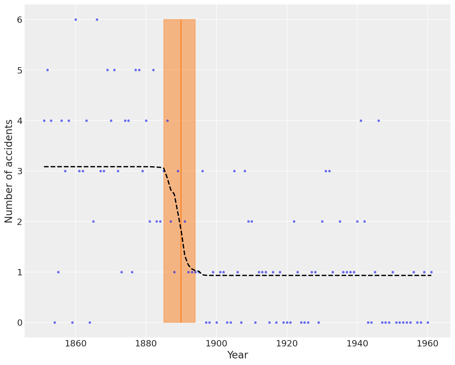
This comprehensive plot shows:

• The observed disaster counts (blue dots)
• The mean switchpoint estimate (orange vertical line) at year ~1890
• The 94% HPD interval for the switchpoint (orange shaded band) spanning approximately 1885-1894
• The expected disaster rate that adapts to the switchpoint (dashed black line)

The expected rate line clearly shows the transition from higher disaster frequency in the early period (averaging ~3 disasters/year) to lower frequency in the later period (averaging ~1 disaster/year). This dramatic reduction is consistent with improvements in mining safety regulations and practices that were implemented in the late 19th century.

Imputed missing values

The dataset contains missing observations for two years: 1890 and 1934. PyMC automatically created latent variables to model these missing values and sampled them as part of the inference process. You can access the imputed values from the posterior:

# Imputed missing values (posterior predictive)
with disasters_model:
    ppc = pm.sample_posterior_predictive(trace, var_names=["obs"], random_seed=42)

# The missing values are stored in idata.posterior['disasters_unobserved']
# ppc["obs"] has shape (draws, years). For missing-year index i, summarize ppc["obs"][ :, i]

Because PyMC created latent variables for missing entries (accessible as disasters_unobserved in the trace), the posterior predictive draws include draws for those years and give an imputed distribution. This allows us to:

• Estimate the likely number of disasters in the missing years
• Quantify our uncertainty about those estimates
• Use the complete dataset for prediction and model checking

The missing data points are particularly interesting: 1890 falls right at the estimated switchpoint, while 1934 is well into the late period with lower disaster rates.

Practical tips

• Discrete parameters cannot be handled by gradient-based samplers. Use a mixture of samplers (Metropolis / CompoundStep + NUTS) or marginalize discrete parameters analytically if possible.
• For short time series with small counts, the Poisson model is appropriate. For over-dispersed data consider a Negative Binomial likelihood instead.
• Visualize the posterior on the switch-point as a histogram (or rug plot over years) to see the probable change interval, not a single point estimate.
• Use posterior predictive checks to confirm the model reproduces the shape and variability of the data.

Extensions

• Allow multiple change-points (e.g., two or more): discrete combinatorics grow quickly; hierarchical priors and reversible-jump approaches are possible but more advanced.
• Model seasonality or covariates: include time-varying covariates or a latent Gaussian process for a smoothly varying rate.
• Marginalize discrete parameters: in some conjugate models you can sum/integrate out the discrete variable analytically to keep everything continuous.

Next steps

For advanced topics like creating custom operations and distributions in PyMC, see PyMC 201: Advanced Topics.

Summary

Change-point models are an excellent first application of Bayesian techniques for count time series. This case study demonstrates how PyMC handles missing observations and how to combine samplers to infer discrete parameters. The coal-mining disasters example remains a compact and instructive problem for learning these techniques.

Key takeaways:

• Mixed sampling strategies allow us to handle models with both discrete and continuous parameters
• Missing data is handled automatically by PyMC when you pass arrays with NaN values
• pm.math.switch provides differentiable conditional logic for piecewise functions
• Convergence diagnostics (r_hat, ESS) are essential for validating MCMC results
• Visualization of the change-point and HDI intervals helps communicate uncertainty

The model successfully identified a significant reduction in coal mining disasters around 1890, corresponding to improved safety regulations in the late 19th century.