Bayesian variable selection through regularization offers an elegant alternative to stepwise regression or ad-hoc feature engineering. This post walks through a complete horseshoe prior implementation in PyMC 5.26.1, demonstrating how global and local shrinkage parameters automatically identify relevant predictors while pushing irrelevant coefficients toward zero.
The problem: multivariate regression with uncertain predictors
We’re working with data from the Listening and Spoken Language Data Repository (LSL-DR), tracking educational outcomes for children with hearing loss. The dataset includes ten potential predictors:
male: gender indicatorsiblings: number of siblings in householdfamily_inv: index of family involvementnon_english: primary household language is not Englishprev_disab: presence of a previous disabilitynon_white: race indicatorage_test: age at testing (months)non_severe_hl: hearing loss is not severemother_hs: mother obtained high school diploma or betterearly_ident: hearing impairment identified by 3 months
The outcome is a standardized test score. Unlike simple linear regression, we don’t know a priori which predictors matter. Classical approaches—stepwise selection, LASSO, ridge regression—shrink coefficients toward zero via penalties. The Bayesian version uses priors to encode the same intuition: most coefficients should be small or zero, but a few may be substantial.
Loading and preprocessing the data
import arviz as az
import matplotlib.pyplot as plt
import numpy as np
import pandas as pd
import pymc as pm
import pytensor.tensor as pt

RANDOM_SEED = 8927
rng = np.random.default_rng(RANDOM_SEED)

# Load data
test_scores = pd.read_csv(pm.get_data("test_scores.csv"), index_col=0)

# Drop missing values and standardize
X = test_scores.dropna().astype(float)
y = X.pop("score")

X -= X.mean()
X /= X.std()

N, D = X.shape  # N observations, D predictors
The first few rows show the structure:
| score | male | siblings | family_inv | non_english | prev_disab | age_test | non_severe_hl | mother_hs | early_ident | non_white |
|---|---|---|---|---|---|---|---|---|---|---|
| 40 | 0 | 2.0 | 2.0 | False | NaN | 55 | 1.0 | NaN | False | False |
| 31 | 1 | 0.0 | NaN | False | 0.0 | 53 | 0.0 | 0.0 | False | False |
| 83 | 1 | 1.0 | 1.0 | True | 0.0 | 52 | 1.0 | NaN | False | True |
Standardizing the features ensures coefficients are on comparable scales, making shrinkage priors more interpretable.
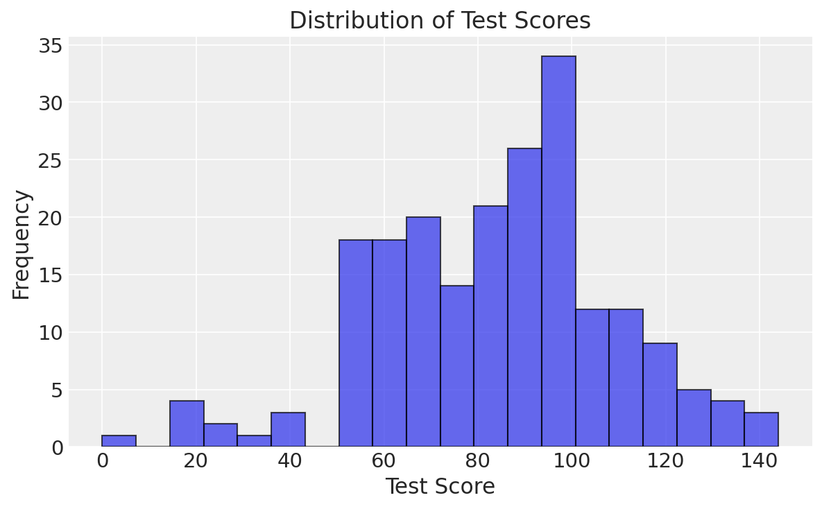
The distribution of test scores shows a roughly normal spread centered around 85-90, with some lower-scoring outliers:
The hierarchical regularized horseshoe prior
The horseshoe prior is a Bayesian regularization strategy that uses heavy-tailed distributions to achieve automatic variable selection. Each coefficient $\beta_i$ gets its own variance controlled by global and local shrinkage:
$$ \beta_i \sim \mathcal{N}\left(0, \tau^2 \cdot \lambda_i^2\right), $$where:
- $\tau$ is the global shrinkage parameter, controlling overall sparsity
- $\lambda_i$ is the local shrinkage parameter for predictor $i$, allowing individual flexibility
Global shrinkage: the $\tau$ parameter
For the global shrinkage, we use a Half-StudentT distribution:
$$ \tau \sim \text{Half-StudentT}_2\left(\frac{D_0}{D - D_0}, \frac{\sigma}{\sqrt{N}}\right), $$where $D_0$ is the expected number of non-zero coefficients. This prior encodes our belief about sparsity: if we expect only half the predictors to matter, set $D_0 = D/2$. The heavy tails allow flexibility if the data demand more active coefficients.
Local shrinkage: the $\lambda_i$ parameters
Each coefficient gets its own local shrinkage term, also from a heavy-tailed distribution:
$$ \lambda_i \sim \text{Half-StudentT}_2(1). $$To prevent over-shrinkage, we introduce a regularized version:
$$ \tilde{\lambda}_i^2 = \frac{c^2 \lambda_i^2}{c^2 + \tau^2 \lambda_i^2}, $$with $c^2 \sim \text{InverseGamma}(1, 1)$. This ratio keeps local shrinkage bounded, preventing coefficients from being forced to exactly zero when they shouldn’t be.
Non-centered reparameterization
To help NUTS navigate the posterior efficiently, we reparameterize the coefficients:
$$ \begin{align} z_i &\sim \mathcal{N}(0, 1), \\ \beta_i &= z_i \cdot \tau \cdot \tilde{\lambda}_i. \end{align} $$Why this matters: The centered parameterization $\beta_i \sim \mathcal{N}(0, \tau^2 \tilde{\lambda}_i^2)$ creates strong posterior correlations between $\beta_i$ and its scale parameters. When $\tau$ and $\tilde{\lambda}_i$ are uncertain, the geometry becomes a narrow funnel that stalls gradient-based samplers. The non-centered version decouples the sampling:
- $z_i$ is explored on a fixed standard normal (easy geometry)
- Scale parameters $\tau$ and $\tilde{\lambda}_i$ update independently
- Posterior correlations vanish, eliminating funnel pathologies
This pattern appears in hierarchical models, variational autoencoders, and any setting where a parameter’s scale is learned. If you see divergences or funnel shapes in trace plots, try non-centered parameterization.
Implementing the model in PyMC
We use named dimensions to keep track of which coefficient corresponds to which predictor:
D0 = int(D / 2)  # Expect half the predictors to be active

with pm.Model(coords={"predictors": X.columns.values}) as test_score_model:
    # Prior on error SD
    sigma = pm.HalfNormal("sigma", 25)

    # Global shrinkage prior
    tau = pm.HalfStudentT("tau", 2, D0 / (D - D0) * sigma / np.sqrt(N))

    # Local shrinkage prior
    lam = pm.HalfStudentT("lam", 5, dims="predictors")
    c2 = pm.InverseGamma("c2", 1, 1)

    # Non-centered parameterization
    z = pm.Normal("z", 0.0, 1.0, dims="predictors")

    # Shrunken coefficients
    beta = pm.Deterministic(
        "beta",
        z * tau * lam * pt.sqrt(c2 / (c2 + tau**2 * lam**2)),
        dims="predictors"
    )

    # No shrinkage on intercept
    beta0 = pm.Normal("beta0", 100, 25.0)

    # Likelihood
    scores = pm.Normal(
        "scores",
        beta0 + pt.dot(X.values, beta),
        sigma,
        observed=y.values
    )
Key implementation details:
coords={"predictors": X.columns.values}labels each dimension with the actual feature namedims="predictors"tells PyMC to create one parameter per predictorpm.Deterministictracks $\beta$ in the trace for diagnostics, even though it’s computed from $z$- The intercept
beta0gets a separate, non-regularized prior
The model structure visualizes the hierarchical relationships:
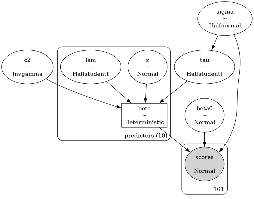
This directed acyclic graph shows how priors flow into the likelihood through the deterministic transformation of coefficients.
Prior predictive checks
Before fitting, simulate from the prior to ensure it generates plausible outcomes:
with test_score_model:
    prior_samples = pm.sample_prior_predictive(100)
Plotting prior predictive scores alongside observed data confirms the prior is reasonable—if prior samples are wildly off-scale, revise the hyperparameters.
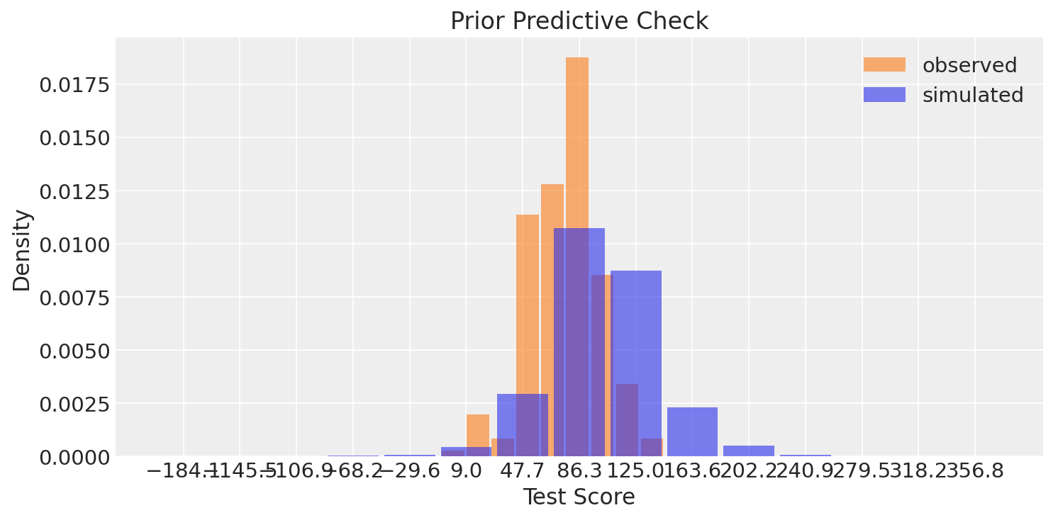
The prior distribution (blue) covers the range of observed scores (orange), indicating our priors are not overly constraining. The prior allows for both higher and lower scores than observed, giving the likelihood room to learn from the data.
Sampling the posterior
Run NUTS with a higher target_accept to reduce divergences from the complex geometry:
with test_score_model:
    idata = pm.sample(1000, tune=2000, random_seed=42, target_accept=0.99)
Sampling strategy:
draws=1000: posterior samples per chaintune=2000: adaptation steps to find good step sizestarget_accept=0.99: stricter acceptance rate to avoid divergences in narrow regions
Convergence diagnostics ($\hat{R} \approx 1$, high ESS) confirm the sampler successfully explored the posterior. If you encounter divergences, increase target_accept or verify the non-centered parameterization is correct.
Interpreting the results
Posterior summary statistics
The posterior estimates reveal clear shrinkage patterns:
| Parameter | Mean | SD | HDI 3% | HDI 97% | ESS Bulk | $\hat{R}$ |
|---|---|---|---|---|---|---|
| beta[family_inv] | -8.293 | 2.171 | -12.506 | -4.388 | 3529.8 | 1.002 |
| beta[prev_disab] | -3.523 | 1.895 | -6.760 | 0.161 | 3447.7 | 1.001 |
| beta[non_english] | -2.623 | 1.724 | -5.780 | 0.374 | 3564.3 | 1.002 |
| beta[early_ident] | 2.849 | 1.774 | -0.243 | 6.106 | 2955.0 | 1.001 |
| beta[non_white] | -2.126 | 1.768 | -5.568 | 0.769 | 3264.9 | 1.002 |
| beta[non_severe_hl] | 1.618 | 1.637 | -1.249 | 4.690 | 3107.6 | 1.000 |
| beta[siblings] | -1.023 | 1.486 | -4.007 | 1.588 | 3968.2 | 1.000 |
| beta[age_test] | 0.623 | 1.415 | -1.871 | 3.636 | 4173.5 | 1.001 |
| beta[male] | 0.600 | 1.328 | -1.661 | 3.481 | 4218.4 | 1.001 |
| beta[mother_hs] | 0.400 | 1.428 | -2.307 | 3.340 | 4519.6 | 1.000 |
| beta0 | 87.834 | 1.798 | 84.522 | 91.304 | 4272.0 | 1.004 |
| tau | 7.550 | 19.405 | 1.081 | 17.519 | 1731.3 | 1.003 |
| sigma | 18.370 | 1.391 | 15.877 | 20.997 | 3613.5 | 1.001 |
| c2 | 112.200 | 986.303 | 2.261 | 228.010 | 2015.2 | 1.002 |
Key findings:
- Family involvement (
beta[family_inv]= -8.3) has the strongest negative effect—higher family involvement scores are associated with lower test scores, which may seem counterintuitive but could reflect measurement artifacts or confounding - Early identification (
beta[early_ident]= 2.8) shows a positive effect, though the HDI barely excludes zero - Previous disability and non-English predictors show negative associations
- The last three predictors (
age_test,male,mother_hs) are effectively shrunk to zero—their HDIs comfortably include zero and their means are small
All $\hat{R}$ values are close to 1.0 and ESS values exceed 1700, confirming excellent convergence.
Global and local shrinkage parameters
The trace plots for tau, sigma, and c2 show well-mixed chains with no divergences:
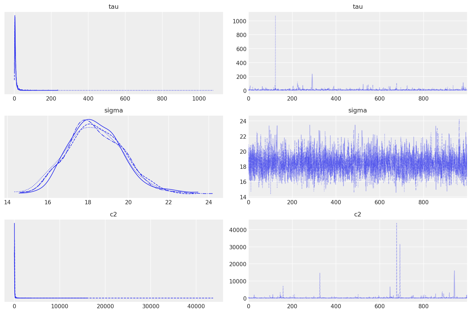
These hyperparameters control how aggressively coefficients are regularized:
tau(global shrinkage) has a posterior mean of 7.55 with wide uncertainty—the data support moderate overall shrinkagesigma(residual error) is tightly estimated around 18.4, reflecting consistent measurement noisec2(regularization scale) prevents excessive shrinkage with a heavy-tailed posterior
The trace plots show no trends or sticking, and the marginal distributions are smooth, indicating the sampler explored the posterior efficiently.
Coefficient estimates
A forest plot of beta reveals the shrinkage pattern:
az.plot_forest(idata, var_names=["beta"], combined=True, hdi_prob=0.95, r_hat=True)
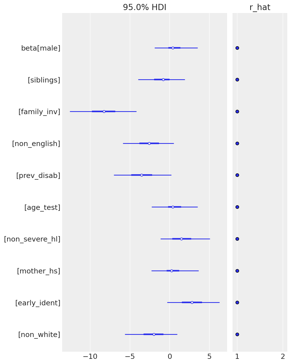
What to look for:
- Family involvement, previous disability, and non-English have 95% HDIs that exclude or barely touch zero (bolded in the table above)—these are credibly non-zero predictors
- Early identification and non-severe hearing loss show moderate effects with wide intervals
- The remaining coefficients (age, male, mother’s education) are tightly shrunk near zero—their HDIs span zero symmetrically
Named dimensions (predictors) ensure each coefficient is labeled with its feature name, making interpretation straightforward. The forest plot’s $\hat{R}$ annotations (all ≈ 1.0) confirm convergence for every coefficient.
Energy plot diagnostics
az.plot_energy(idata)
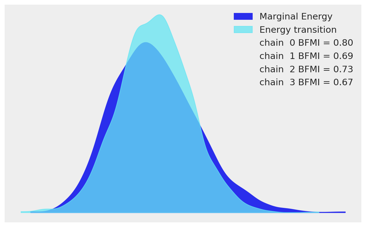
The energy plot compares the distribution of energy levels during sampling (E-BFMI diagnostic). The marginal energy distribution (histograms on sides) and transition energy distribution (central curve) show good separation, indicating NUTS is exploring the posterior efficiently. Well-separated distributions confirm the sampler is not getting stuck in narrow regions. The absence of overlap suggests no pathological geometry—our non-centered parameterization worked as intended.
Practical workflow tips
Start with informative $D_0$: Set the expected number of active coefficients based on domain knowledge or exploratory analysis. Being within an order of magnitude is sufficient.
Monitor divergences: If you see warnings, increase
target_acceptto 0.99 or higher. Persistent divergences may signal model misspecification or prior-data conflict.Use named dimensions early: Passing
coordsanddimsupfront makes diagnostics and posterior summaries self-documenting.Validate with posterior predictive checks: After sampling, generate posterior predictive samples and compare to observed data to verify fit quality.
Compare with simpler models: Fit a non-regularized regression as a baseline. If the horseshoe model doesn’t improve LOO or posterior predictive accuracy, the added complexity may not be justified.
When to use the horseshoe prior
The horseshoe excels when:
- You have many predictors and expect only a subset to be relevant
- You want automatic selection without manual stepwise procedures
- Interpretability matters: coefficients retain their original scale, unlike penalized methods that mix regularization into the loss function
It’s less effective when:
- All predictors genuinely contribute (no sparsity)
- Strong multicollinearity is present (shrinkage can be unstable)
- Computation time is critical (horseshoe models are slower than ridge or LASSO)
Extensions and next steps
The hierarchical regularized horseshoe is one of many sparsity-inducing priors. Related approaches include:
- Finnish horseshoe: alternative parameterization with tighter theoretical guarantees
- Spike-and-slab: discrete mixture prior for binary inclusion indicators
- Regularized R² prior: targets a specific proportion of explained variance
For deeper theory, see Piironen & Vehtari (2017) on the regularized horseshoe. For implementation patterns, the PyMC example gallery includes more variable selection case studies.
What we learned from the LSL-DR analysis
The horseshoe prior successfully identified a sparse set of active predictors from ten candidates:
Strong predictors (95% HDI excludes or barely touches zero):
- Family involvement index (large negative effect)
- Previous disability status (negative)
- Non-English primary language (negative)
Moderate predictors (wide HDIs, plausible effects):
- Early identification of hearing loss (positive trend)
- Non-severe hearing loss (positive trend)
Shrunk to zero (effectively excluded):
- Age at testing
- Gender
- Mother’s education
- Number of siblings
- Race
This automatic selection happened without stepwise procedures or manual feature engineering—the prior structure did the work. The model suggests that socioeconomic and disability-related factors dominate educational outcomes in this cohort, while demographic variables contribute little once those factors are accounted for.
Cautions: The counterintuitive negative coefficient for family involvement warrants scrutiny. This could reflect:
- Reverse causation (families engage more when children struggle)
- Measurement artifacts (how “involvement” is coded)
- Confounding with unmeasured variables
These findings should motivate follow-up analyses with causal inference methods or sensitivity tests, not immediate policy recommendations.
Summary
The hierarchical regularized horseshoe prior automates variable selection by shrinking irrelevant coefficients toward zero while leaving important ones unpenalized. Key techniques—non-centered reparameterization, named dimensions, and careful tuning of target_accept—ensure efficient sampling and interpretable results. This workflow scales to high-dimensional regression problems where manual feature selection is impractical, making it a valuable tool in the Bayesian modeling toolkit.