JAX 203: Probabilistic Programming with Bamojax

Welcome to JAX 203! This lab follows the content/ipynb/jax_203.ipynb notebook and shows how to express a Beta–Bernoulli coin model in Bamojax, run BlackJax’s No-U-Turn Sampler (NUTS), and sanity-check the posterior with predictive simulations.

0. Environment setup

Imports and plotting style configuration match the notebook exactly; run them first to make sure Bamojax, BlackJax, and Matplotlib are available.

import jax.numpy as jnp
import jax.random as jr
import numpy as np
import matplotlib.pyplot as plt
import numpyro.distributions as dist

from bamojax.base import Model
from bamojax.samplers import mcmc_sampler
from bamojax.inference import MCMCInference

from blackjax import nuts

plt.style.use("seaborn-v0_8-darkgrid")

1. Data

The dataset is a short run of biased coin flips. Converting it to jax.numpy keeps everything on the accelerator (or CPU) that BlackJax will use later.

coin_flips = jnp.array(
    [1, 1, 1, 1, 1, 1, 1, 1, 1, 1, 1, 1, 1, 0, 0, 1, 0, 1, 1, 0],
    dtype=jnp.int32,
)
num_trials = int(coin_flips.size)
successes = int(coin_flips.sum())
failures = num_trials - successes

print(f"Observed {successes} heads and {failures} tails out of {num_trials} flips.")

Observed 16 heads and 4 tails out of 20 flips.

2. Build the model

Bamojax represents probabilistic programs as graphs of Node instances. The notebook places a uniform Beta prior on the latent coin weight and attaches a Bernoulli likelihood to each observation.

model = Model(name="Beta-Bernoulli coin")

theta = model.add_node("theta", distribution=dist.Beta(1.0, 1.0))
likelihood = model.add_node(
    "y",
    distribution=dist.Bernoulli,
    observations=coin_flips,
    parents={"probs": theta},
    shape=coin_flips.shape,
)

print("Latent nodes:", list(model.get_latent_nodes().keys()))
print("Leaf node:", [node.name for node in model.get_leaf_nodes()])

Latent nodes: ['theta']
Leaf node: ['y']

3. Configure and run NUTS

With the model defined, Bamojax’s mcmc_sampler helper wires the graph into a BlackJax NUTS transition kernel. The inference object runs 500 burn-in iterations, 500 warmup steps, and retains 2 000 samples for posterior analysis.

initial_kernel = mcmc_sampler(
    model,
    mcmc_kernel=nuts,
    mcmc_parameters={"step_size": 0.1, "inverse_mass_matrix": jnp.array([1.0])},
)

inference = MCMCInference(
    model=model,
    num_chains=1,
    mcmc_kernel=initial_kernel,
    num_samples=2000,
    num_burn=500,
    num_warmup=500,
    return_diagnostics=True,
)

rng_key = jr.PRNGKey(2)

print("Running NUTS sampling (first call may compile JAX kernels)...")
results = inference.run(rng_key)

theta_samples = results["states"]["theta"]
diagnostics = results["info"]

print(f"Collected {theta_samples.shape[0]} posterior samples.")
print(f"Average acceptance rate: {float(diagnostics.acceptance_rate.mean()):.3f}")

Running NUTS sampling (first call may compile JAX kernels)...
Adapting NUTS HMC parameters... done.
Collected 2000 posterior samples.
Average acceptance rate: 0.891

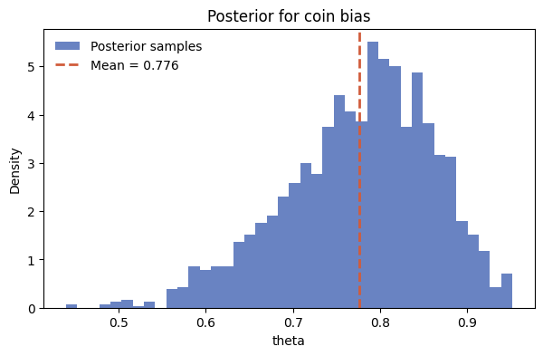
4. Posterior summary

Posterior expectations, credible intervals, and conjugate checks line up with Beta–Bernoulli intuition: strong evidence that the coin is biased toward heads.

theta_np = np.asarray(theta_samples)
posterior_mean = theta_np.mean()
posterior_ci = np.quantile(theta_np, [0.025, 0.5, 0.975])
prob_theta_gt_half = (theta_np > 0.5).mean()

posterior_alpha = 1.0 + successes
posterior_beta = 1.0 + failures

print(f"Posterior mean: {posterior_mean:.3f}")
print(f"Central 95% interval: [{posterior_ci[0]:.3f}, {posterior_ci[2]:.3f}]")
print(f"P(theta > 0.5 | data) = {prob_theta_gt_half:.3f}")
print(
    f"Conjugate Beta parameters (reference): alpha={posterior_alpha:.1f}, "
    f"beta={posterior_beta:.1f}"
)

Posterior mean: 0.776
Central 95% interval: [0.589, 0.917]
P(theta > 0.5 | data) = 0.998
Conjugate Beta parameters (reference): alpha=17.0, beta=5.0

fig, ax = plt.subplots(figsize=(7, 4))
ax.hist(
    theta_np,
    bins=40,
    color="#4f6db8",
    alpha=0.85,
    density=True,
    label="Posterior samples",
)
ax.axvline(
    posterior_mean,
    color="#d05c3b",
    linestyle="--",
    linewidth=2,
    label=f"Mean = {posterior_mean:.3f}",
)
ax.set(xlabel="theta", ylabel="Density", title="Posterior for coin bias")
ax.legend(frameon=False)
fig.savefig("static/img/jax203/posterior_hist.png", bbox_inches="tight")

Posterior for coin bias

5. Posterior predictive checks

Sampling new datasets from the posterior confirms that the observed number of heads is typical under the model.

num_ppc_draws = 200
ppc_keys = jr.split(jr.PRNGKey(4), num_ppc_draws)
theta_subset = np.asarray(theta_samples[-num_ppc_draws:])

posterior_predictive_counts = []
for subkey, theta_value in zip(ppc_keys, theta_subset):
    state = {"theta": jnp.array(theta_value)}
    simulated = model.sample_predictive(subkey, state)["y"]
    posterior_predictive_counts.append(np.asarray(simulated).sum())

posterior_predictive_counts = np.asarray(posterior_predictive_counts)
ppc_interval = np.quantile(posterior_predictive_counts, [0.025, 0.975])

print(f"Posterior predictive mean heads: {posterior_predictive_counts.mean():.2f}")
print(
    "Posterior predictive 95% interval for heads: "
    f"[{ppc_interval[0]:.1f}, {ppc_interval[1]:.1f}]"
)

Posterior predictive mean heads: 16.02
Posterior predictive 95% interval for heads: [12.0, 20.0]

fig, ax = plt.subplots(figsize=(7, 4))
bins = np.arange(-0.5, num_trials + 1.5, 1)
ax.hist(
    posterior_predictive_counts,
    bins=bins,
    color="#5aa469",
    alpha=0.85,
    rwidth=0.9,
)
ax.axvline(
    successes,
    color="#d05c3b",
    linestyle="--",
    linewidth=2,
    label=f"Observed heads = {successes}",
)
ax.set(
    xlabel="Number of heads out of 20",
    ylabel="Frequency",
    title="Posterior predictive distribution",
)
ax.set_xticks(range(0, num_trials + 1, 2))
ax.legend(frameon=False)
fig.savefig("static/img/jax203/posterior_predictive.png", bbox_inches="tight")

Posterior predictive distribution

6. Next steps

Swap in alternative priors (e.g., Beta(2, 2)) to see how strongly posterior mass reacts compared with the conjugate baseline.
Replicate the workflow with a Binomial likelihood instead of Bernoulli observations to practice changing Bamojax node wiring.
Port the posterior draws into ArviZ or corner plots for convergence diagnostics beyond the acceptance rate.

References

Max Hinne. 2025. Bamojax: Bayesian Modelling with JAX. Journal of Open Source Software, 10(114), 8642. https://doi.org/10.21105/joss.08642