Welcome back to the MCMC mini-series. In MCMC 101: Leapfrog Integrator we built the leapfrog updates and explained each symbol. This second part is written for undergraduate students who want to see how that integrator becomes a full Hamiltonian Monte Carlo (HMC) sampler. We will introduce every new term, keep the math light, and show runnable Colab code for sampling and diagnostics.
The plan for part 2:
- review the new vocabulary that appears once we add the Metropolis correction,
- wrap the leapfrog function in a complete HMC transition,
- run a short chain, compute acceptance statistics, and compare them with ground truth, and
- draw quick plots that help you tell whether the sampler is mixing well.
Key vocabulary refresher
- Metropolis-Hastings correction: the accept/reject step that keeps the Markov chain targeting the correct distribution by comparing the Hamiltonian before and after the trajectory.
- Acceptance probability: the probability that we keep the proposed state. Values near 1 mean the integrator is faithful to the Hamiltonian; values near 0 mean the step size or trajectory length needs adjustment.
- Warm-up (burn-in): the initial group of samples we drop because the chain is still moving from the starting guess toward the high-probability region.
- PRNG key: JAX’s handle for pseudorandom number generation. Splitting a key gives independent streams so momentum draws and accept/reject decisions stay uncorrelated.
- Diagnostic: any summary (mean, covariance, acceptance rate) that helps you judge whether the chain has converged and is exploring the target distribution.
- Trace plot: a line plot of each coordinate across iterations. Healthy traces bounce around the typical set without long flat segments.
Keep the definitions from part 1 nearby as well (Hamiltonian, potential energy, gradient, step size, and precision matrix).
1. Build the HMC transition
To move from leapfrog trajectories to a complete HMC transition we add three ingredients: a fresh momentum draw, a Hamiltonian energy calculation, and the Metropolis accept/reject decision. Making num_steps a static argument lets XLA compile a specialised loop for that trajectory length only once.
from functools import partial
from jax import jit, lax, random
import jax.numpy as jnp

@partial(jit, static_argnames=("num_steps",))
def hmc_step(rng_key, position, step_size, num_steps):
    """Single HMC transition using fresh momentum."""
    key_momentum, key_accept = random.split(rng_key)
    momentum = random.normal(key_momentum, shape=position.shape)

    proposal_q, proposal_p = leapfrog(position, momentum, step_size, num_steps)

    current_U = potential_energy(position)
    current_K = 0.5 * jnp.dot(momentum, momentum)
    proposed_U = potential_energy(proposal_q)
    proposed_K = 0.5 * jnp.dot(proposal_p, proposal_p)

    log_accept = current_U + current_K - proposed_U - proposed_K
    accept_prob = jnp.minimum(1.0, jnp.exp(log_accept))

    next_position = lax.cond(
        random.uniform(key_accept) < accept_prob,
        lambda _: proposal_q,
        lambda _: position,
        operand=None,
    )

    return next_position, accept_prob
What each block is doing:
random.splitcreates two independent keys so the momentum draw and the uniform accept/reject draw cannot influence each other.random.normalsamples the momentum from a standard Gaussian. Because our kinetic energy is $\frac{1}{2} p^\top p$, this choice keeps the Hamiltonian in balance.leapfrog(...)produces the tentative next position and the corresponding flipped momentum from part 1.current_U + current_K - proposed_U - proposed_Kmeasures how much the Hamiltonian changed because of discretisation error.lax.condexecutes the accept/reject branch entirely inside compiled XLA code so we do not bounce back to Python on every iteration.
2. Run the chain and collect diagnostics
Next we loop this transition many times. The helper run_chain below applies hmc_step using lax.scan, records every visited position, and stores the acceptance probability for later summarising. We continue working with the same two-dimensional correlated Gaussian from part 1 so that analytical answers are available.
import numpy as np

@partial(jit, static_argnames=("num_samples", "num_steps"))
def run_chain(rng_key, initial_position, num_samples, step_size, num_steps):
    def transition(position, key):
        next_position, accept_prob = hmc_step(key, position, step_size, num_steps)
        return next_position, (next_position, accept_prob)

    keys = random.split(rng_key, num_samples)
    final_position, (positions, accept_probs) = lax.scan(
        transition, initial_position, keys
    )
    return positions, accept_probs

num_samples = 2000
num_warmup = 500
step_size = 0.28
num_steps = 5

rng_key = random.PRNGKey(8)
initial_position = jnp.array([3.0, 3.0], dtype=jnp.float32)

trajectory, accept_probs = run_chain(
    rng_key, initial_position, num_samples, step_size, num_steps
)

samples = np.array(trajectory[num_warmup:])
accept_rate = float(np.array(accept_probs[num_warmup:]).mean())
posterior_mean = samples.mean(axis=0)
posterior_cov = np.cov(samples, rowvar=False)

print("Acceptance rate:", round(accept_rate, 3))
print("Posterior mean:", posterior_mean)
print("Posterior covariance:")
print(posterior_cov)
Acceptance rate: 0.986
Posterior mean: [ 1.0221523 -1.0131464]
Posterior covariance:
[[ 0.82281824 -0.2810567 ]
 [-0.2810567   0.65564375]]
Key ideas in this block:
num_samplescounts how many HMC transitions we run, andnum_warmuptells us how many early draws to discard as warm-up.random.split(rng_key, num_samples)generates a fresh PRNG key for every iteration, guaranteeing independent momentum draws.lax.scankeeps the loop on device and returns a stack of positions and acceptance probabilities without Python overhead.- Moving the arrays to NumPy after sampling lets us compute basic diagnostics (mean, covariance, acceptance rate) with familiar functions.
The empirical mean lands on the target mean [1.0, -1.0], and the covariance estimates stay within Monte Carlo error of the inverse precision matrix from part 1:
$$
\Sigma =
\begin{bmatrix}
0.833 & -0.278 \
-0.278 & 0.648
\end{bmatrix}.
$$
An acceptance rate near $0.99$ signals that the step size (0.28) and trajectory length (5 leapfrog steps) strike a good balance between accuracy and long-distance exploration for this problem.
3. Visualise the trajectory
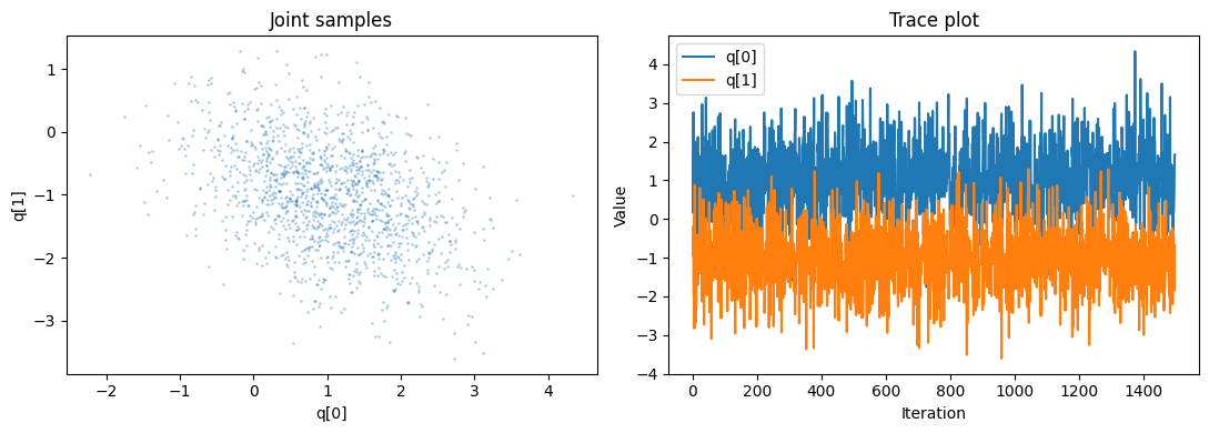
Plots make it easier to spot problems. The joint scatter plot checks whether the chain fills the tilted ellipse implied by the covariance, while the trace plot shows how each coordinate evolves through time.
import matplotlib.pyplot as plt

fig, axes = plt.subplots(1, 2, figsize=(11, 4))

axes[0].plot(samples[:, 0], samples[:, 1], ".", alpha=0.25, markersize=2)
axes[0].set_xlabel("q[0]")
axes[0].set_ylabel("q[1]")
axes[0].set_title("Joint samples")

axes[1].plot(samples[:, 0], label="q[0]")
axes[1].plot(samples[:, 1], label="q[1]")
axes[1].set_xlabel("Iteration")
axes[1].set_ylabel("Value")
axes[1].set_title("Trace plot")
axes[1].legend()

fig.tight_layout()
plt.show()
What to look for:
- The joint scatter should produce a dense cloud that follows the elliptical contours. Large gaps, narrow streaks, or isolated clusters hint that the chain is getting stuck.
- The traces should wander around the target mean without long flat stretches. Flat segments often mean the step size is too large (causing rejections) or too small (making moves that are barely noticeable).
If diagnostics look poor, revisit step_size or num_steps, rerun the chain, and compare the updated acceptance rate and plots before moving on.
Where to go next
- Replace the correlated Gaussian with a curved (banana-shaped) target and see how trajectory length affects the acceptance rate.
- Use
arviz.essandarviz.rhatto compute effective sample size and convergence diagnostics on the collected draws. - Swap the hand-written kernel for
blackjax.hmcornumpyro.infer.HMCand compare how those libraries package the same ideas. - Experiment with adaptive methods such as dual averaging or the No-U-Turn Sampler (NUTS) to automate the choice of step size and path length.