Welcome to JAX 202! After exploring vectorization and multi-device training, it is time to lean into probabilistic inference. BlackJax builds on core JAX primitives to provide Hamiltonian Monte Carlo (HMC), No-U-Turn Sampler (NUTS), and adaptive algorithms that jit into tight sampling loops. This guide shows how to go from a log-density function to converged posterior draws without leaving the JAX ecosystem.
You will learn how to (1) define targets as pure JAX functions, (2) set up BlackJax kernels and initial states, (3) run a quick warmup heuristic to tune step size and mass matrices, (4) vectorize chains for throughput, and (5) monitor diagnostics such as effective sample size (ESS) and the Gelman-Rubin statistic.
0. Environment setup
Install the probabilistic stack inside the same Colab or workstation environment used for previous lessons. You need BlackJax plus supporting libraries for transformations, diagnostics, and data prep.
%pip install -q -U "jax[cpu]" blackjax arviz optax scikit-learn
If GPUs are available, swap "jax[cpu]" for "jax[cuda12_pip]" to reuse accelerator support. BlackJax compiles kernels with jit, so ensure your environment tracks JAX ≥ 0.4.30 to avoid deprecation warnings. In Colab, verify accelerator access with !nvidia-smi or the runtime status badge before you start tracing kernels.
1. Load a real dataset in Colab
Google Colab ships with scikit-learn, so you can tap into curated datasets without uploading files. The Wisconsin Breast Cancer dataset provides 30 standardized features and a binary target—perfect for logistic regression benchmarks.
import numpy as np
from sklearn.datasets import load_breast_cancer
from sklearn.model_selection import train_test_split
from sklearn.preprocessing import StandardScaler

dataset = load_breast_cancer(as_frame=False)
features, labels = dataset.data, dataset.target.astype(np.float32)

x_train_np, x_test_np, y_train_np, y_test_np = train_test_split(
    features,
    labels,
    test_size=0.2,
    random_state=0,
    stratify=labels,
)

scaler = StandardScaler()
x_train_np = scaler.fit_transform(x_train_np)
x_test_np = scaler.transform(x_test_np)
Convert the NumPy arrays into JAX arrays so the sampler stays on-device. Keep hold-out splits for posterior predictive checks.
import jax
import jax.numpy as jnp

train_features = jnp.asarray(x_train_np)
train_labels = jnp.asarray(y_train_np)
test_features = jnp.asarray(x_test_np)
test_labels = jnp.asarray(y_test_np)
Confirm that JAX sees at least one device and that the GPU runtime is active when available.
jax.device_count()
1
jax.default_backend()
'gpu'
2. Framing the posterior
BlackJax expects a callable returning the log-probability of the target distribution. Keep the function side-effect free and operate purely on JAX arrays.
def logistic_regression_logprob(theta, x, y):
    weight, bias = theta[:-1], theta[-1]
    logits = jnp.dot(x, weight) + bias
    log_likelihood = jnp.sum(y * logits - jnp.logaddexp(0.0, logits))
    log_prior = -0.5 * jnp.sum(theta**2)  # standard normal prior
    return log_likelihood + log_prior
For binary labels $y_i \in {0, 1}$ with feature vectors $x_i \in \mathbb{R}^d$, the logistic regression log-likelihood is
$$ \log p(\mathbf{y} \mid \theta, X) = \sum_{i=1}^{N}\left[y_i \cdot (x_i^\top w + b) - \log\left(1 + e^{x_i^\top w + b}\right)\right], $$
where $\theta = (w, b)$. The standard normal prior on the parameters contributes
$$ \log p(\theta) = -\tfrac{1}{2},\theta^\top \theta - \tfrac{d_\theta}{2} \log(2\pi), $$
with $d_\theta = \dim(\theta) = d + 1$. In code we drop the constant $-\tfrac{d_\theta}{2} \log(2\pi)$ because BlackJax only needs the log-density up to an additive constant.
Combining both terms yields the log-posterior $\log p(\theta \mid X, \mathbf{y}) = \log p(\mathbf{y} \mid \theta, X) + \log p(\theta)$ that feeds into BlackJax.
Batch your data as host arrays or ShapedArray placeholders. The signature should be (params, *data) so that you can partially apply data and differentiate with respect to parameters.
from functools import partial

target_logprob = partial(logistic_regression_logprob, x=train_features, y=train_labels)
Because BlackJax pulls gradients via jax.grad, any nondifferentiable operations inside target_logprob will surface immediately as FilteredStackTrace errors—fix them before continuing.
3. Initializing kernels and states
blackjax.hmc returns a functional pair of init and step. Wrap it in a helper so you can rebuild the sampler with new hyperparameters during tuning.
import blackjax

num_integration_steps = 10
dimension = train_features.shape[1] + 1

def build_hmc(step_size, inverse_mass_matrix):
    return blackjax.hmc(
        logdensity_fn=target_logprob,
        step_size=step_size,
        inverse_mass_matrix=inverse_mass_matrix,
        num_integration_steps=num_integration_steps,
    )

step_size = 1e-2
inverse_mass_matrix = jnp.ones(dimension)
hmc = build_hmc(step_size, inverse_mass_matrix)
init_state = hmc.init(jnp.zeros(dimension))
init_state stores the current position, momentum, and potential energy. The identity inverse mass matrix seeds HMC with unit variances; you will refine it once warmup statistics accumulate. To carry auxiliary data (e.g., running acceptance stats), unpack and re-pack the state each iteration—BlackJax structures are PyTrees, so they cooperate with jit and pmap.
4. Sampling in a compiled loop
Use jax.lax.fori_loop or jax.lax.scan to iterate hmc.step. Keep randomness threaded through the loop so each step sees an independent momentum refresh.
def sample_hmc(hmc, rng_key, state, num_samples):
    def one_step(carry, _):
        rng_key, state = carry
        rng_key, subkey = jax.random.split(rng_key)
        state, info = hmc.step(subkey, state)
        return (rng_key, state), (state.position, info)

    (_, final_state), (positions, infos) = jax.lax.scan(
        one_step, (rng_key, state), xs=None, length=num_samples
    )
    return positions, infos, final_state
Because everything is pure JAX, the first call traces the full sampling loop, and subsequent calls with the same shapes run at compiled speed. Avoid Python-side lists or conditional logging inside one_step; use jax.debug.print sparingly if divergence counts spike.
5. Manual warmup with quick heuristics
Colab’s preinstalled BlackJax (≥1.0) no longer ships a blackjax_default warmup, so run a few short pilot batches to adjust the step size and diagonal mass matrix yourself. The quick heuristic below shrinks the step size when acceptance falls under 75% and grows it when acceptance exceeds 85%.
def tune_hmc(rng_key, state, step_size, inverse_mass_matrix, num_rounds=6, batch_size=256):
    log_history = []
    for round_id in range(num_rounds):
        hmc = build_hmc(step_size, inverse_mass_matrix)
        rng_key, round_key = jax.random.split(rng_key)
        positions, infos, state = sample_hmc(hmc, round_key, state, num_samples=batch_size)
        accept_rate = float(jnp.mean(infos.is_accepted))

        if accept_rate < 0.75:
            step_size *= 0.8
        elif accept_rate > 0.85:
            step_size *= 1.2

        centered = positions - jnp.mean(positions, axis=0)
        variances = jnp.mean(centered**2, axis=0) + 1e-3
        inverse_mass_matrix = 1.0 / variances

        log_history.append((round_id, accept_rate, step_size))

    final_hmc = build_hmc(step_size, inverse_mass_matrix)
    return final_hmc, state, inverse_mass_matrix, log_history, rng_key

rng_key = jax.random.key(0)
hmc, state, inverse_mass_matrix, warmup_log, rng_key = tune_hmc(
    rng_key,
    init_state,
    step_size=step_size,
    inverse_mass_matrix=inverse_mass_matrix,
)

rng_key, draw_key = jax.random.split(rng_key)
positions, infos, state = sample_hmc(hmc, draw_key, state, num_samples=2000)
posterior_draws = positions
The simple schedule records acceptance each round in warmup_log so you can inspect convergence. Increase num_rounds or batch_size if acceptance fluctuates wildly; dial back the adjustment multipliers when you prefer gentler updates.
6. Vectorizing multiple chains
To launch several chains, vmap the init/step functions over independent seeds and initial positions. BlackJax kernels are reentrant, making vmap or pmap straightforward.
chain_ids = jnp.arange(4)
chain_keys = jax.random.split(rng_key, len(chain_ids))
chain_positions = state.position + 0.01 * jax.vmap(
    lambda key: jax.random.normal(key, state.position.shape)
)(chain_keys)

@jax.vmap
def run_chain(rng_key, initial_position):
    state = hmc.init(initial_position)
    samples, infos, _ = sample_hmc(hmc, rng_key, state, num_samples=1000)
    return samples, infos

samples, infos = run_chain(chain_keys, chain_positions)
posterior_draws = samples.reshape(-1, dimension)
With pmap, place the outer axis on devices to split chains across GPUs. Keep per-chain sample counts identical so the compiled graph remains static.
7. Monitoring diagnostics
Collect kernel metadata (acceptance rates, energy errors) from infos and feed samples to ArviZ for summary statistics.
import arviz as az

idata = az.from_dict(
    posterior={"theta": samples},
    sample_stats={
        "accept_prob": infos.is_accepted,
        "energy": infos.energy,
    },
    dims={"theta": ["theta_dim"]},
)

summary = az.summary(idata, var_names=["theta"], kind="diagnostics")
print(summary[["ess_bulk", "r_hat"]])

stats_summary = az.summary(idata, var_names=["theta"], kind="stats")
print("\nStats Summary:")
print(stats_summary[["mean", "sd", "hdi_3%", "hdi_97%"]])
           ess_bulk  r_hat
theta[0]      152.0   1.03
theta[1]      616.0   1.01
theta[2]      291.0   1.01
theta[3]       76.0   1.09
theta[4]      383.0   1.00
theta[5]      271.0   1.01
theta[6]      358.0   1.02
theta[7]      171.0   1.01
theta[8]      872.0   1.00
theta[9]      244.0   1.01
theta[10]     114.0   1.00
theta[11]     690.0   1.01
theta[12]     178.0   1.01
theta[13]      90.0   1.03
theta[14]     853.0   1.00
theta[15]     384.0   1.01
theta[16]     339.0   1.02
theta[17]     392.0   1.01
theta[18]     549.0   1.00
theta[19]     255.0   1.01
theta[20]      56.0   1.06
theta[21]     477.0   1.02
theta[22]     183.0   1.01
theta[23]     115.0   1.03
theta[24]     421.0   1.00
theta[25]     252.0   1.01
theta[26]     234.0   1.02
theta[27]     237.0   1.01
theta[28]     629.0   1.00
theta[29]     209.0   1.01
theta[30]     557.0   1.00

Stats Summary:
            mean     sd  hdi_3%  hdi_97%
theta[0]  -0.661  0.919  -2.440    0.975
theta[1]  -0.579  0.590  -1.618    0.583
theta[2]  -0.567  0.902  -2.316    1.063
theta[3]  -0.894  0.967  -2.828    0.862
theta[4]  -0.232  0.625  -1.433    0.914
theta[5]   0.428  0.761  -1.039    1.760
theta[6]  -0.860  0.800  -2.378    0.620
theta[7]  -1.040  0.823  -2.650    0.502
theta[8]   0.117  0.559  -0.902    1.143
theta[9]   0.572  0.726  -0.716    1.983
theta[10] -1.552  0.797  -3.048   -0.061
theta[11]  0.008  0.520  -0.953    0.992
theta[12] -0.781  0.834  -2.436    0.714
theta[13] -1.067  0.973  -2.877    0.825
theta[14] -0.319  0.520  -1.244    0.713
theta[15]  0.676  0.717  -0.680    1.971
theta[16]  0.211  0.607  -0.927    1.337
theta[17] -0.402  0.697  -1.713    0.869
theta[18]  0.530  0.587  -0.594    1.603
theta[19]  0.620  0.714  -0.602    2.000
theta[20] -1.206  0.934  -2.838    0.585
theta[21] -1.112  0.649  -2.295    0.197
theta[22] -0.903  0.893  -2.699    0.622
theta[23] -0.887  0.897  -2.602    0.806
theta[24] -0.851  0.639  -2.063    0.320
theta[25] -0.323  0.838  -1.869    1.232
theta[26] -0.830  0.771  -2.282    0.536
theta[27] -0.944  0.807  -2.430    0.509
theta[28] -0.949  0.575  -2.020    0.100
theta[29] -0.586  0.733  -1.929    0.780
theta[30]  0.322  0.447  -0.491    1.187

Visual checks complement numeric diagnostics. Plot the first four parameters and make sure each chain explores the same support.

```python
import matplotlib.pyplot as plt

az.plot_trace(
    idata,
    var_names=["theta"],
    coords={"theta_dim": slice(0, 4)},
    compact=True,
    figsize=(10, 6),
)
plt.tight_layout()
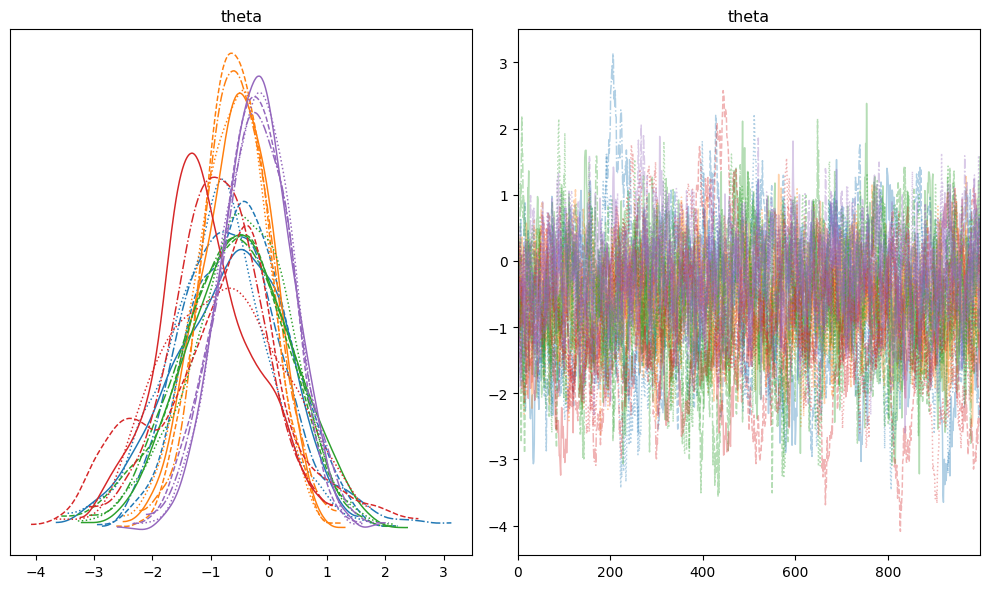
Watch for:
- Low ESS: Increase trajectory length (
num_integration_steps) or re-run warmup with a denser mass matrix. r_hat> 1.01: Seed more chains or extend the sampling run until Gelman-Rubin diagnostics stabilize.- Divergences: Reduce step size and warm up again; divergences indicate energy discrepancies from the integrator.
To evaluate predictive accuracy on the held-out split, convert posterior draws into logits, average them, and compute class probabilities.
def posterior_predictive_mean(theta_samples, x):
    logits = x @ theta_samples[..., :-1].T + theta_samples[..., -1]
    mean_logit = jnp.mean(logits, axis=-1)
    return jax.nn.sigmoid(mean_logit)

theta_samples = posterior_draws.reshape(-1, train_features.shape[1] + 1)
probs = posterior_predictive_mean(theta_samples, test_features)
pred_labels = (probs > 0.5).astype(jnp.int32)
test_accuracy = jnp.mean(pred_labels == test_labels)
print(f"Posterior predictive accuracy: {test_accuracy * 100:.1f}%")
Posterior predictive accuracy: 98.2%
8. Beyond basic kernels
- Try
blackjax.nutsfor path-length adaptation that removes the need to choosenum_integration_steps. - Swap in
blackjax.rmh(randomized midpoint integrator) when you need higher-order accuracy on challenging posteriors. - Combine BlackJax with TFP JAX distributions or custom bijectors to reparameterize constrained variables.
- For online inference, roll your own
jax.lax.scanthat interleaves streaming data updates with kernel steps.
With the BlackJax toolbox, you can express rich probabilistic models while staying inside the jit/pmap-friendly subset of JAX. Practice on small datasets, watch diagnostics, and scale out once you trust your sampler.