Welcome to JAX 102! In JAX 101 we wrote a full training loop with jit, grad, and vmap. This installment dives into the jax.lax module - the place where you reach for structured control flow that plays nicely with XLA compilation, reverse-mode autodiff, and device parallelism.
If you have ever written a Python for loop, if statement, or while loop inside a JAX function and seen a warning about tracer values, this guide is for you. The goal is to replace eager Python control flow with staged lax primitives without giving up readability.
0. Notebook setup
Spin up the same Colab or local environment from 101. The only new import is jax.lax, which ships with JAX itself.
import jax
import jax.numpy as jnp
from jax import lax, jit, grad
Throughout the notebook we wrap examples in jit so you can see which patterns compile without surprises.
1. Why lax control flow exists
Python executes loops and conditionals on the host interpreter. As soon as you close over tracer values (the symbolic placeholders JAX uses when staging computations), vanilla control flow breaks because the interpreter needs concrete values to decide which branch to run or how many iterations to perform.
jax.lax primitives encode the same intent, but they leave the decision-making to XLA, which lowers the whole program into a single fused graph. That means:
- You can pass loop bounds, predicates, or branch conditions that depend on JAX arrays.
- The resulting function is differentiable:
gradandjacfwdsee through the loop body. jitcompiles once, regardless of the input data that flows through the branches.
Keep that framing in mind as we tour the four most common primitives.
2. Deterministic loops with lax.fori_loop
lax.fori_loop(lower, upper, body_fn, init_val) mirrors a Python for loop that iterates from lower (inclusive) to upper (exclusive). The loop carries a value through each iteration and returns the final state.
def dot_fori_loop(a, b):
    """Compute a dot product with lax.fori_loop to expose the mechanics."""
    def body_fun(i, carry):
        acc = carry + a[i] * b[i]
        return acc

    return lax.fori_loop(0, a.shape[0], body_fun, 0.0)

a = jnp.array([1., 2., 3., 4.])
b = jnp.array([-1., 0.5, 0.25, 2.])
print("Python dot :", jnp.dot(a, b))
print("lax.fori_loop dot:", dot_fori_loop(a, b))
Python dot : 8.5
lax.fori_loop dot: 8.5
The loop index i is a plain integer, but the carry (acc) can be any PyTree - arrays, dictionaries, tuples, and more. Because the bounds are static integers, this form is ideal for fixed-size loops like neural-network layers where you know the iteration count a priori.
You can JIT and differentiate the function without additional work:
dot_grad = grad(lambda x: dot_fori_loop(x, b))
print("Gradient wrt a:", dot_grad(a))
Gradient wrt a: [-1. 0.5 0.25 2. ]
3. Stateful scans with lax.scan
lax.scan generalizes fori_loop to both carry state forward and emit a sequence of intermediate results. Reach for it whenever you would normally accumulate values in a list or run a recurrent model.
def exponential_moving_average(x, alpha=0.1):
    """Return EMA values for a 1D signal using lax.scan."""
    def body(carry, x_t):
        prev = carry
        ema = (1 - alpha) * prev + alpha * x_t
        return ema, ema  # new carry, value to collect

    init = x[0]
    ema_values, _ = lax.scan(body, init, x[1:])
    return jnp.concatenate([jnp.array([init]), ema_values])

signal = jnp.linspace(0., 1., 6)
print("Signal:", signal)
print("EMA   :", exponential_moving_average(signal))
Signal: [0.  0.2 0.4 0.6 0.8 1. ]
EMA   : [0.    0.02  0.058 0.1322 0.23898 0.375082]
The function consumes the tail of the signal (x[1:]), maintaining the current EMA as the carry and returning each updated EMA in the output sequence. Because everything is vectorized and staged, you can safely wrap exponential_moving_average in jit or take gradients with respect to the smoothing factor alpha.
scan also accepts reverse=True and length= arguments for more advanced patterns, and it fuses the loop body into a single XLA op that can run on accelerators without additional ceremony.
4. Dynamic stopping with lax.while_loop
When the number of iterations depends on runtime data, move to lax.while_loop(cond_fun, body_fun, init_val). The condition and body operate on the same carry PyTree. JAX guarantees the loop terminates when cond_fun first returns False.
def newton_sqrt(x, max_iters=25, tol=1e-6):
    """Use lax.while_loop to run Newton iterations until convergence."""
    def cond_fn(state):
        iter_idx, y, err = state
        return jnp.logical_and(iter_idx < max_iters, err > tol)

    def body_fn(state):
        iter_idx, y, _ = state
        y_next = 0.5 * (y + x / y)
        err = jnp.abs(y_next**2 - x)
        return (iter_idx + 1, y_next, err)

    init = (0, x, jnp.abs(x - x))
    _, estimate, _ = lax.while_loop(cond_fn, body_fn, init)
    return estimate

value = 7.0
print("sqrt via lax.while_loop:", newton_sqrt(value))
print("jax.numpy.sqrt        :", jnp.sqrt(value))
sqrt via lax.while_loop: 2.6457512
jax.numpy.sqrt        : 2.6457512
Because the loop state is a tuple, you can track metadata like iteration counters or residuals alongside the running estimate. This pattern shows up in optimization, root finding, and sampler warm-up. Everything is differentiable with respect to x, so you can embed Newton iterations inside larger autodiff pipelines.
5. Branching with lax.cond and lax.switch
Branches in JAX must evaluate both sides eagerly unless you use conditional primitives. lax.cond(pred, true_operand, true_fun, false_operand, false_fun) only executes the branch that matches the predicate. Operands can be any PyTree you want to feed into the branch function.
def safe_log(x):
    """Return log(x) with a fallback when x <= 0, fully JIT-compatible."""
    return lax.cond(
        x > 0,
        x,
        lambda v: jnp.log(v),
        x,
        lambda v: -jnp.inf,
    )

vals = jnp.array([2.0, 1.0, 1e-3, 0.0, -4.0])
print("safe_log:", jax.vmap(safe_log)(vals))
safe_log: [ 0.6931472 0. -6.9077554 -inf -inf]
For multi-way branching, use lax.switch(index, branch_fns, operand), where branch_fns is a tuple of callables and index selects which to evaluate. Both primitives keep the computation inside the JAX trace so you can nest them inside jit or grad.
6. Composing lax with jit and grad
lax primitives behave like any other JAX function, so you can freely compose them with transformations. The example below builds a toy recurrent cell whose hidden state updates via scan, while the batch dimension is vectorized with vmap. We then JIT-compile the whole inference function.
def rnn_step(carry, x_t, params):
    h_prev = carry
    w_hh, w_xh = params
    h = jnp.tanh(h_prev @ w_hh + x_t @ w_xh)
    return h, h

def run_rnn(inputs, params):
    h0 = jnp.zeros((params[0].shape[0],))
    final_h, outputs = lax.scan(lambda c, x: rnn_step(c, x, params), h0, inputs)
    return final_h, outputs

def batched_run_rnn(batch_inputs, params):
    return jax.vmap(lambda seq: run_rnn(seq, params))(batch_inputs)

jitted_run = jit(batched_run_rnn)

key = jax.random.PRNGKey(0)
params = (
    jax.random.normal(key, (8, 8)),
    jax.random.normal(key, (4, 8)),
)
batch = jax.random.normal(key, (3, 16, 4))
final_states, activations = jitted_run(batch, params)
print("final_states shape:", final_states.shape)
print("activations shape :", activations.shape)
final_states shape: (3, 8)
activations shape : (3, 16, 8)
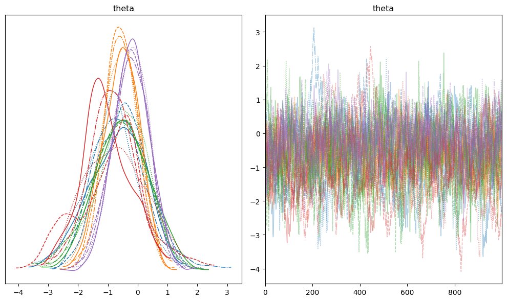
7. Visual diagnostics after lax-driven sampling
The sampling loops in JAX 202 rely on lax.scan to propagate Hamiltonian Monte Carlo states. Once you have an InferenceData object, you can visualize chain mixing without leaving the JAX trace:
import matplotlib.pyplot as plt

az.plot_trace(
    idata,
    var_names=["theta"],
    coords={"theta_dim": slice(0, 4)},
    compact=True,
    figsize=(10, 6),
)
plt.tight_layout()
Because all control flow is expressed with lax, jit sees a single static computation graph. Gradients with respect to params or the inputs flow automatically:
loss = lambda p: jitted_run(batch, p)[0].sum()
print("dLoss/dw_hh shape:", grad(loss)(params)[0].shape)
dLoss/dw_hh shape: (8, 8)
8. Debugging and gotchas
laxprimitives require pure functions. Avoid Python side effects such as appending to lists or mutating globals; use carry states instead.- Shapes must be consistent across branches and loop iterations. XLA needs static signatures to compile; mismatched shapes trigger shape errors at trace time.
- Prefer
lax.scanover manualfori_loopwhen you need the intermediate outputs; it fuses faster and uses less memory than accumulating Python lists and stacking afterward. - Combine
jax.debug.printwithlax.condorlax.scanwhen you need to peek at intermediate values without de-optimizing your JIT’ed function.
9. Where to go next
- Swap
lax.scanfor higher-level libraries like Flax’snn.scanif you want parameter sharing across time steps with less boilerplate. - Explore
lax.map,lax.associative_scan, andlax.broadcastto structure parallel-friendly loops. - Revisit the logistic regression from 101 and migrate the gradient-descent loop to
lax.fori_loopto see how it transforms underjit.
You now have the control-flow vocabulary needed to keep JAX programs both expressive and compilable. In the next installment we will load real datasets and use these primitives to structure larger training pipelines.