Perceptron 102: Classification with Neural Networks

In Perceptron 101, we built a single perceptron for regression. Now we extend it to classification—predicting discrete categories instead of continuous values. The key insight: add an activation function to transform linear outputs into probabilities.

The Classification Problem

Consider sentences containing only two words: aack and beep. Count each word ($x_1$ and $x_2$), and classify:

• If more “beep” ($x_2 > x_1$): classify as “angry” (red)
• Otherwise: classify as “happy” (blue)

This is a binary classification problem with linearly separable classes.

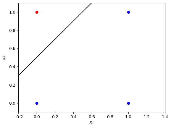
The line $x_1 - x_2 + 0.5 = 0$ separates the classes. Our goal: find parameters $w_1$, $w_2$, and $b$ for $w_1x_1 + w_2x_2 + b = 0$ as a decision boundary.

Why Activation Functions?

For regression, the perceptron output is $\hat{y} = Wx + b$. But classification needs outputs between 0 and 1 (probabilities). The sigmoid function provides this:

Combined with the linear transformation:

We predict class 1 (red) if $a > 0.5$, otherwise class 0 (blue).

The Log Loss Cost Function

For classification, we use log loss instead of sum of squares:

This penalizes confident wrong predictions heavily, which is exactly what we want for classification.

Implementation

The structure remains almost identical to regression—only forward propagation and cost computation change.

Sigmoid Function

def sigmoid(z):
    return 1 / (1 + np.exp(-z))

print("sigmoid(-2) =", sigmoid(-2))   # 0.119
print("sigmoid(0) =", sigmoid(0))     # 0.5
print("sigmoid(3.5) =", sigmoid(3.5)) # 0.971

Modified Forward Propagation

def forward_propagation(X, parameters):
    W = parameters["W"]
    b = parameters["b"]
    
    # Forward Propagation with sigmoid activation
    Z = np.matmul(W, X) + b
    A = sigmoid(Z)
    
    return A

Log Loss Cost Function

def compute_cost(A, Y):
    m = Y.shape[1]
    
    logprobs = - np.multiply(np.log(A), Y) - np.multiply(np.log(1 - A), 1 - Y)
    cost = 1/m * np.sum(logprobs)
    
    return cost

Backward Propagation

Remarkably, the gradient formulas are the same as regression:

def backward_propagation(A, X, Y):
    m = X.shape[1]
    
    dZ = A - Y
    dW = 1/m * np.dot(dZ, X.T)
    db = 1/m * np.sum(dZ, axis=1, keepdims=True)
    
    grads = {"dW": dW, "db": db}
    return grads

Training Results

Generate a simple dataset with 30 examples:

m = 30
X = np.random.randint(0, 2, (2, m))
Y = np.logical_and(X[0] == 0, X[1] == 1).astype(int).reshape((1, m))

Train for 50 iterations:

parameters = nn_model(X, Y, num_iterations=50, learning_rate=1.2, print_cost=True)

Cost after iteration 0: 0.693480
Cost after iteration 10: 0.346813
Cost after iteration 20: 0.243080
Cost after iteration 30: 0.188716
Cost after iteration 40: 0.154382
Cost after iteration 49: 0.132574

The resulting decision boundary cleanly separates the two classes:

Making Predictions

def predict(X, parameters):
    A = forward_propagation(X, parameters)
    predictions = A > 0.5
    return predictions

X_pred = np.array([[1, 1, 0, 0],
                   [0, 1, 0, 1]])
Y_pred = predict(X_pred, parameters)

print(f"Predictions: {Y_pred}")
# [[False False False  True]]

Only the point (0, 1) is predicted as class 1 (red)—exactly as expected.

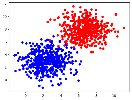
Scaling to Larger Datasets

Using sklearn.datasets.make_blobs for a more complex dataset:

from sklearn.datasets import make_blobs

samples, labels = make_blobs(n_samples=1000, 
                             centers=([2.5, 3], [6.7, 7.9]), 
                             cluster_std=1.4,
                             random_state=0)

X_larger = np.transpose(samples)
Y_larger = labels.reshape((1, 1000))

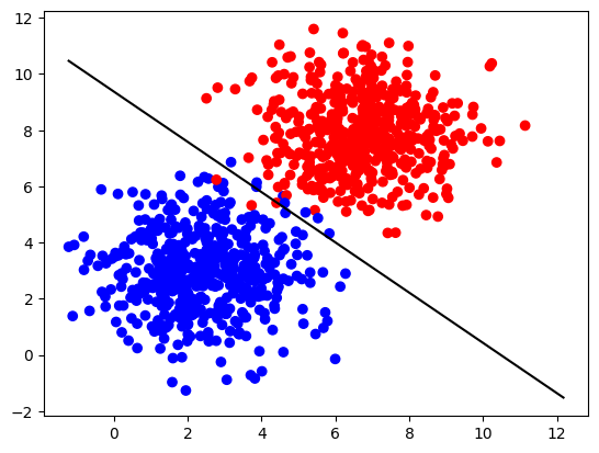
After training for 100 iterations:

parameters_larger = nn_model(X_larger, Y_larger, num_iterations=100, learning_rate=1.2)
print("W =", parameters_larger["W"])  # [[1.016 1.137]]
print("b =", parameters_larger["b"])  # [[-10.65]]

The decision boundary successfully separates the two clusters:

Key Takeaways

1. Activation functions enable classification: The sigmoid transforms linear outputs to probabilities in [0, 1].

2. Log loss is ideal for classification: It heavily penalizes confident wrong predictions, unlike squared error.

3. Same gradient formulas: Despite different cost functions, the gradients $\frac{\partial \mathcal{L}}{\partial W}$ and $\frac{\partial \mathcal{L}}{\partial b}$ have the same form as regression.

4. Threshold at 0.5: Predictions use $a > 0.5$ to assign class labels.

5. Linearly separable classes: A single perceptron can only learn linear decision boundaries. For complex patterns, you need multiple layers.

Next Steps

• Explore other activation functions (ReLU, tanh)
• Add hidden layers for non-linear decision boundaries
• Implement multi-class classification with softmax
• Apply regularization to prevent overfitting

The perceptron with sigmoid activation is the foundation of logistic regression and the building block for deeper neural networks.