Linear regression feels deceptively simple until you re-implement it from scratch using a neural network. The C2_W3_Lab_1_regression_with_perceptron.ipynb notebook demonstrates how a single perceptron can solve both simple and multiple linear regression problems. This post distills that implementation into a practical reference for understanding how neural networks learn linear relationships.
Why Start With a Perceptron?
A perceptron is the simplest building block of neural networks—a single node that takes weighted inputs, adds a bias, and produces an output. For linear regression, the perceptron output is simply:
$$\hat{y} = wx + b$$where $w$ is the weight, $x$ is the input, and $b$ is the bias. The beauty of this approach is that you can train it using gradient descent, just like more complex networks.
Simple Linear Regression: TV Marketing to Sales
The Problem
Given TV marketing expenses, predict sales. The dataset has 200 examples with two fields:
TV: marketing budget in thousandsSales: sales in thousands
Data Exploration
import numpy as np
import pandas as pd
import matplotlib.pyplot as plt

np.random.seed(3)

adv = pd.read_csv("tvmarketing.csv")
print(adv.head())
Output:
      TV  Sales
0  230.1   22.1
1   44.5   10.4
2   17.2    9.3
3  151.5   18.5
4  180.8   12.9
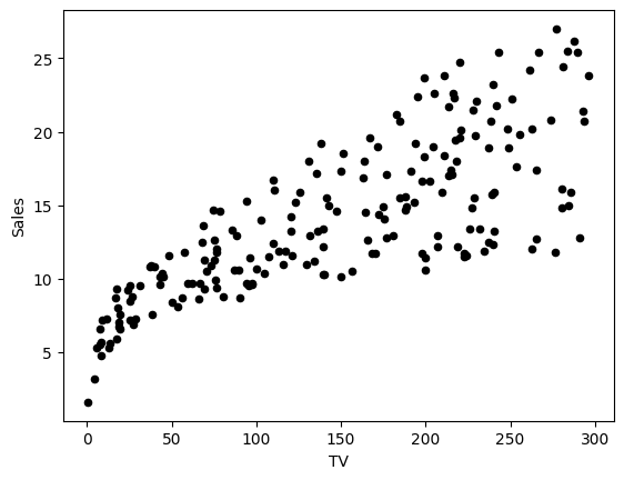
The scatter plot shows a clear positive linear relationship between TV marketing budget and sales:
Data Normalization
Before training, normalize the features by subtracting the mean and dividing by standard deviation:
adv_norm = (adv - np.mean(adv)) / np.std(adv)

X_norm = np.array(adv_norm['TV']).reshape((1, len(adv_norm)))
Y_norm = np.array(adv_norm['Sales']).reshape((1, len(adv_norm)))

print(f'The shape of X_norm: {X_norm.shape}')  # (1, 200)
print(f'The shape of Y_norm: {Y_norm.shape}')  # (1, 200)
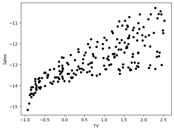
After normalization, the data maintains the same linear pattern but with standardized scales:
Neural Network Implementation
The implementation follows a clean structure:
1. Define Network Structure
def layer_sizes(X, Y):
    """
    Returns:
        n_x -- input layer size
        n_y -- output layer size
    """
    n_x = X.shape[0]
    n_y = Y.shape[0]
    return (n_x, n_y)
2. Initialize Parameters
def initialize_parameters(n_x, n_y):
    """Initialize weights with small random values, bias with zeros"""
    W = np.random.randn(n_y, n_x) * 0.01
    b = np.zeros((n_y, 1))

    parameters = {"W": W, "b": b}
    return parameters
3. Forward Propagation
def forward_propagation(X, parameters):
    """Calculate predictions: Y_hat = WX + b"""
    W = parameters["W"]
    b = parameters["b"]

    Z = np.matmul(W, X) + b
    Y_hat = Z
    return Y_hat
4. Compute Cost
The cost function measures prediction error using sum of squares:
$$\mathcal{L}(w, b) = \frac{1}{2m}\sum_{i=1}^{m} (\hat{y}^{(i)} - y^{(i)})^2$$def compute_cost(Y_hat, Y):
"""Compute sum of squares cost function"""
m = Y_hat.shape[1]
cost = np.sum((Y_hat - Y)**2) / (2*m)
return cost
5. Backward Propagation
Calculate gradients for gradient descent:
$$\frac{\partial \mathcal{L}}{\partial w} = \frac{1}{m}\sum_{i=1}^{m} (\hat{y}^{(i)} - y^{(i)})x^{(i)}$$$$\frac{\partial \mathcal{L}}{\partial b} = \frac{1}{m}\sum_{i=1}^{m} (\hat{y}^{(i)} - y^{(i)})$$def backward_propagation(Y_hat, X, Y):
"""Calculate gradients with respect to W and b"""
m = X.shape[1]
dZ = Y_hat - Y
dW = (1/m) * np.dot(dZ, X.T)
db = (1/m) * np.sum(dZ, axis=1, keepdims=True)
grads = {"dW": dW, "db": db}
return grads
6. Update Parameters
def update_parameters(parameters, grads, learning_rate=1.2):
    """Apply gradient descent updates"""
    W = parameters["W"] - learning_rate * grads["dW"]
    b = parameters["b"] - learning_rate * grads["db"]

    parameters = {"W": W, "b": b}
    return parameters
7. Complete Training Loop
def nn_model(X, Y, num_iterations=10, learning_rate=1.2, print_cost=False):
    """
    Train the neural network model

    Returns:
        parameters -- learned weights and bias
    """
    n_x, n_y = layer_sizes(X, Y)
    parameters = initialize_parameters(n_x, n_y)

    for i in range(num_iterations):
        # Forward propagation
        Y_hat = forward_propagation(X, parameters)

        # Compute cost
        cost = compute_cost(Y_hat, Y)

        # Backward propagation
        grads = backward_propagation(Y_hat, X, Y)

        # Update parameters
        parameters = update_parameters(parameters, grads, learning_rate)

        if print_cost:
            print(f"Cost after iteration {i}: {cost:f}")

    return parameters
Training Results
Training with 30 iterations converges quickly:
parameters_simple = nn_model(X_norm, Y_norm, num_iterations=30,
                            learning_rate=1.2, print_cost=True)
The cost decreases from ~82 to near-zero within a few iterations, showing rapid convergence.
Making Predictions
def predict(X, Y, parameters, X_pred):
    """Make predictions and denormalize results"""
    W = parameters["W"]
    b = parameters["b"]

    # Normalize predictions using training stats
    X_mean = X.mean()
    X_std = X.std()
    X_pred_norm = ((X_pred - X_mean) / X_std).reshape((1, len(X_pred)))

    # Forward propagation
    Y_pred_norm = np.matmul(W, X_pred_norm) + b

    # Denormalize
    Y_pred = Y_pred_norm * np.std(Y) + np.mean(Y)
    return Y_pred[0]

X_pred = np.array([50, 120, 280])
Y_pred = predict(adv["TV"], adv["Sales"], parameters_simple, X_pred)
print(f"TV marketing expenses:\\n{X_pred}")
print(f"Predictions of sales:\\n{Y_pred}")
The model produces reasonable predictions aligned with the linear trend. Here’s a visualization of the fitted regression line (red) with prediction points (blue) overlaid on the original data (black):
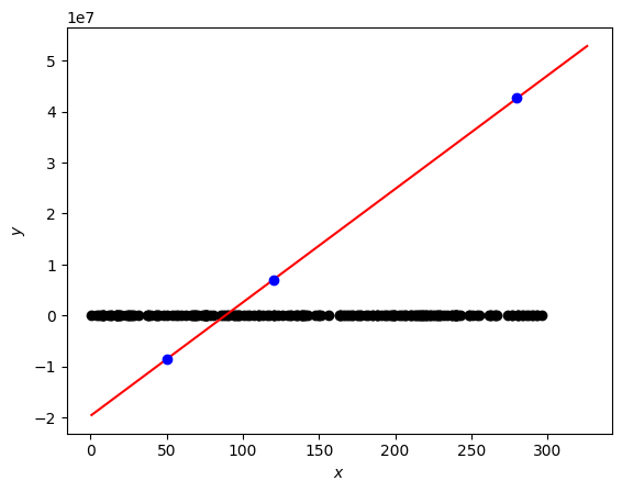
The regression line captures the overall trend well, and the three prediction points fall along the learned line, demonstrating that the perceptron has successfully learned the linear relationship between TV marketing spend and sales.
Multiple Linear Regression: House Prices
Now let’s extend to multiple inputs. The model becomes:
$$\hat{y} = w_1x_1 + w_2x_2 + b = Wx + b$$In matrix form:
$$Z = WX + b$$where $W$ is now a (1×2) matrix and $X$ is (2×m).
The House Prices Dataset
Using the Kaggle House Prices dataset with two features:
GrLivArea: Ground living area (square feet)OverallQual: Overall quality rating (1-10)
df = pd.read_csv('house_prices_train.csv')
X_multi = df[['GrLivArea', 'OverallQual']]
Y_multi = df['SalePrice']

print(X_multi.head())
Output:
   GrLivArea  OverallQual
0       1710            7
1       1262            6
2       1786            7
3       1717            7
4       2198            8
No Code Changes Needed!
The remarkable part: the exact same neural network code works for multiple inputs. Simply reshape the data:
X_multi_norm = (X_multi - np.mean(X_multi)) / np.std(X_multi)
Y_multi_norm = (Y_multi - np.mean(Y_multi)) / np.std(Y_multi)

X_multi_norm = np.array(X_multi_norm).T  # Shape: (2, 1460)
Y_multi_norm = np.array(Y_multi_norm).reshape((1, len(Y_multi_norm)))

print(f'The shape of X: {X_multi_norm.shape}')  # (2, 1460)
print(f'The shape of Y: {Y_multi_norm.shape}')  # (1, 1460)
The gradients automatically extend to matrix operations:
$$\frac{\partial \mathcal{L}}{\partial W} = \frac{1}{m}(\hat{Y} - Y)X^T$$Training Multiple Regression
parameters_multi = nn_model(X_multi_norm, Y_multi_norm,
                           num_iterations=100, print_cost=True)
Making Multi-Feature Predictions
X_pred_multi = np.array([[1710, 7], [1200, 6], [2200, 8]]).T
Y_pred_multi = predict(X_multi, Y_multi, parameters_multi, X_pred_multi)

print(f"Ground living area, square feet: {X_pred_multi[0]}")
print(f"Overall quality ratings: {X_pred_multi[1]}")
print(f"Predicted sales prices: ${np.round(Y_pred_multi)}")
Key Takeaways
Single perceptron = linear regression: A neural network with one node is mathematically equivalent to linear regression.
Gradient descent universality: The same training loop works for any number of inputs—matrix multiplication handles the scaling automatically.
Normalization matters: Standardizing features improves convergence and numerical stability.
Forward-backward pattern: This structure (forward propagation → cost → backward propagation → update) appears in every neural network, regardless of complexity.
From simple to complex: Understanding a single perceptron makes deeper networks intuitive—they’re just more layers of the same building blocks.
Next Steps
- Try polynomial features to capture non-linear relationships
- Add regularization to prevent overfitting
- Experiment with different learning rates
- Extend to classification problems with sigmoid activation
The perceptron is foundational. Master it, and you’ll have the mental model for understanding transformers, CNNs, and beyond.